
Basic Course of Thermo-Fluid Analysis 12: Chapter 5 Basics of thermo-fluid analyses - 5.1 Fundamental equations and discretization
Chapter 5 Basics of thermo-fluid analyses I
This chapter describes basic concepts and procedures for thermo-fluid analyses.
5.1 Fundamental equations and discretization
Transfer or motion of a fluid or heat is expressed by differential equations. For incompressible fluids, which are mainly considered here, the following equations are fundamental:
- Navier-Stokes equations (Momentum equations)
- Equation of continuity
- Energy conservation equation
The Navier-Stokes equations and the continuity equation express the motion of a fluid, while the energy conservation equation expresses the motion of heat. These equations are fundamental for thermo-fluid analyses, and are called governing equations (or fundamental equations ).
If the fundamental equations can be analytically solved, the distributions of heat, temperature, and flow can be explicitly obtained. However, the equations are sufficiently complex and analytic results have only been obtained for very limited cases. As an alternative, thermo-fluid analysis uses the computer to numerically solve the fundamental equations. However, a computer can only process discrete values and cannot process continuous values as is illustrated in the following example.
A calculator can obtain the results of an equation “y = x + 1”, for example, by calculating as follows:
If x = 1, y = 1 + 1 = 2
If x = 2, y = 2 + 1 = 3
If x = 3, y = 3 + 1 = 4
:
:
As shown above, a calculator can obtain a calculation result for discrete input values. However, it cannot process a function, which is a series of continuous or infinitely small values.
To solve this problem, the fundamental equations must be transformed into expressions composed of discrete values. This transformation is called discretization.
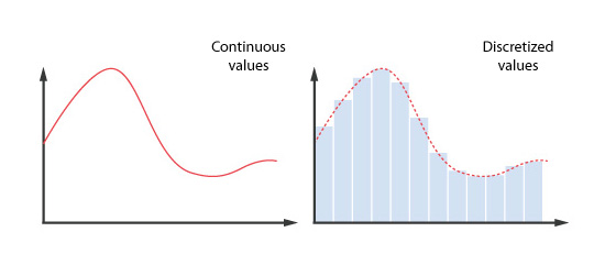
Figure 5.1: Example of discretization
To help understand discretization intuitively, consider the weather. The weather varies continuously in space, so it cannot be easily processed, as is, by computer.
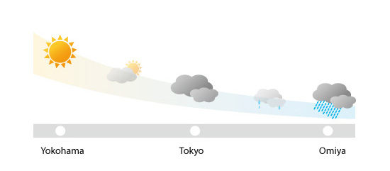
Figure 5.2: Actual weather in three cities
To process the weather using a computer, first determine a specific location where the weather will be characterized. Then, develop relationships that characterize the change in the weather between the specific location identified and the surrounding area. This process corresponds to discretization. Assume the obtained relation is as follows: The weather at any point is given by averaging the weather at surrounding points. According to this relationship, when the weather in Yokohama and Omiya are sunny and rainy, respectively, the computer calculates their average and determines the weather will be “cloudy” in Tokyo.
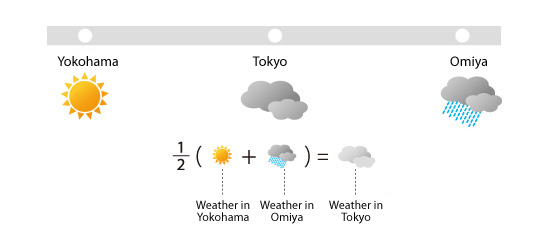
Figure 5.3: Weather processed by computer
A simple average is used in the aforementioned example; however, more complicated relationships are used to describe thermo-fluid relationships between a specific point in space and the surrounding points in a thermo-fluid analysis. There are a few different discretization methods but the major ones are:
Many commercial thermo-fluid software products use the finite volume method for discretization. (The finite volume method is explained in the next chapter.) So while the fundamental thermo-fluid equations are differential equations (which by definition correspond to an infinitesimally small difference between neighboring “points”), discretization enables expressing the relationships between neighboring spaces with algebraic equations (equations that can be expressed using basic arithmetic operations).
To simulate thermo-fluid phenomena such as the flow of the wind around buildings, air flow over a car or the temperature distribution in a room in a thermo-fluid analysis, the target space must be first divided into tiny regions called elements or cells. Then, the fundamental equations for thermo-fluid flow which have been discretized using one of the methods listed above, along with assigning appropriate boundary and initial conditions can be solved numerically. The result is solution of the flow velocity and pressure distributions from the Navier-Stokes and continuity equations, and the temperature from the energy conservation equation.

About the Author
Atsushi Ueyama | Born in September 1983, Hyogo, Japan
He has a Doctor of Philosophy in Engineering from Osaka University. His doctoral research focused on numerical method for fluid-solid interaction problem. He is a consulting engineer at Software Cradle and provides technical support to Cradle customers. He is also an active lecturer at Cradle seminars and training courses.

