5.7 Matrix solver

As seen in the previous section, the parameter values of each element are determined as a function of the values in the neighboring elements. For example, consider Element3 shown in Figure 5.20. The following expression is satisfied.

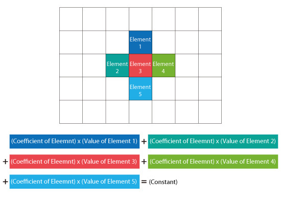
Figure 5.20: Positional relationship of an element with neighboring elements, and the relationship equation

This is a two-dimensional example. Element3 contacts with four total elements on the left, right, top, and bottom. For a three-dimensional example, the neighboring elements of Element3 would be not only the aforementioned four elements but also two more elements at the front and back of Element3. Therefore, for the three-dimensional example, the total number of the neighboring elements is six. For the flow equation, the constant is the external force acting on Element3 while the rate of heating is the constant for the thermal equation.

This relationship equation is created for each element. Therefore, if the model consists of one million elements, one million simultaneous linear equations with one million unknowns per variable would have to be solved. The group of equations can be expressed in matrix form and the solver used to determine the solutions to the equations is called the matrix solver. One of two different solver methods is commonly used. The first method is called the direct method, and the second method is called the iterative method. In a thermo-fluid analysis, the iterative method is generally used. Consider this example. A simultaneous system of linear equations with two unknowns is solved using the Jacobi iterative method.

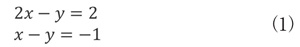
The exact solution to this system of equations is x = 3 and y = 4. For a better understanding of how the solution is obtained iteratively, the system (1) is transformed as shown below:

To solve the system (2) by using the iterative method, give x and y initial values. Here, zero is entered initial values for x and y.

For the first iteration, the solution is x = 1 and y = 1. When this solution is substituted back into system (2) :

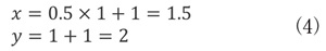
The second iterated solution is x = 1.5 and Y = 2. The process is repeated as shown in Figure 5.1 until the change in the solution values becomes very small, closer to the exact solution.

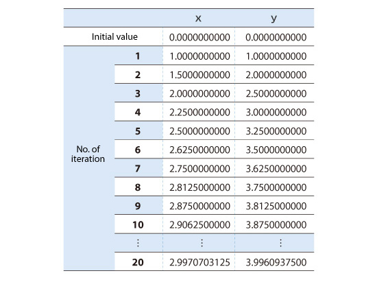
Figure 5.1: Calculation results using Jacobi method

In this example, the Jacobi method was used because of its simplicity. However, for practical problems with millions of elements and requiring hundreds of iterations, higher-speed iterative methods are needed.

As the number of iterations increases, the calculated result gets closer to the exact solution. However, for real world problems, obtaining the exact solution by iterating is difficult to achieve. Therefore, for most problems, the calculations are terminated when the difference between the calculated results for k^-1th and kth calculations is less than a predetermined value. Then, the k^th calculation result is used as the solution. The predetermined value is called the convergence criterion. Be aware that if the calculation does not converge sufficiently, i.e. the difference between the k^-1thand k^th calculations does not approach the convergence criterion, the correct solution may not be obtained.

---

About the Author
Atsushi Ueyama | Born in September 1983, Hyogo, Japan  

He has a Doctor of Philosophy in Engineering from Osaka University. His doctoral research focused on numerical method for fluid-solid interaction problem. He is a consulting engineer at Software Cradle and provides technical support to Cradle customers. He is also an active lecturer at Cradle seminars and training courses.