
Basic Course of Thermo-Fluid Analysis 15: Chapter 5 Basics of thermo-fluid analyses - 5.5 Boundary conditions, 5.6 Initial condition
5.5 Boundary conditions
The value of a parameter within an element is calculated from the values for that parameter in the neighboring elements. For example, in Figure 5.14, the values for the elements shown in blue are used to calculate the value for the element shown in red.
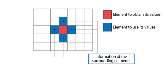
Figure 5.14: Element surrounded by other elements
However, when an element is at the edge of the analysis domain as shown by the red element in Figure 5.15, the value for the element cannot use this method because one of the neighboring elements is missing. In this case, a value must be assigned for each parameter along the edge of the computational domain which corresponds to the edge of the element. The values assigned along the edges of the computational domain are called boundary conditions.
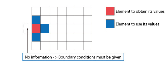
Figure 5.15: Element at the edge of the computational domain
In thermo-fluid analyses, fluid velocity, pressure, and temperature are typical boundary conditions. For example, if the wind is blowing into the computational domain, the values for the wind velocity and inflow temperature are the boundary conditions for the model.
There are three major types of boundary conditions:
・Dirichlet boundary condition
The Dirichlet boundary condition specifies the values of a boundary directly. Conditions such as “Velocity: 5 m/s”, “Pressure: 0 Pa”, and “Temperature: 20°C” are considered Dirichlet boundary conditions.
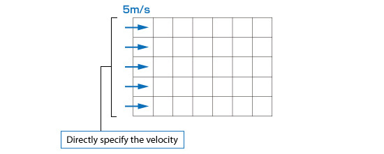
Figure 5.16: Dirichlet boundary condition for a flow
・Neumann boundary condition
The Neumann boundary condition is a condition that specifies the gradient of the parameters. The gradient can be thought of as the rate of change. Conditions such as a free-slip condition and an adiabatic condition are examples of Neumann boundary conditions.
For example, consider an adiabatic condition as shown in (a) of Figure 5.17. When the temperatures at two points are different, heat transfers from the point with higher temperature to the point with the lower temperature. An adiabatic condition means no heat is transferred. This is achieved by having the temperatures of the two points be the same (see [b] of Figure 5.17). When the temperatures of the two points are the same, the temperature gradient (rate of change) is 0. Therefore, an adiabatic condition can be expressed by a Neumann boundary condition with a temperature gradient equal to 0.
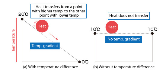
Figure 5.17: Idea of adiabatic condition
・Periodic boundary condition
A periodic boundary condition sets the same values for a parameter on two or more faces. It is used to simulate periodicity (repetition) of the distribution. For the fan shown in Figure 5.18, the fan has four blades equally spaced around the center hub. The flow around each blade should be almost the same for all the blades. A periodic boundary condition can be applied to the boundary faces of one of the blades. This is used to simulate the motion of the entire fan by only modeling one blade. Note that there are certain times when the periodic boundary condition cannot be used. For example, a very high speed flow may not be periodic even though the geometrical model appears periodic.
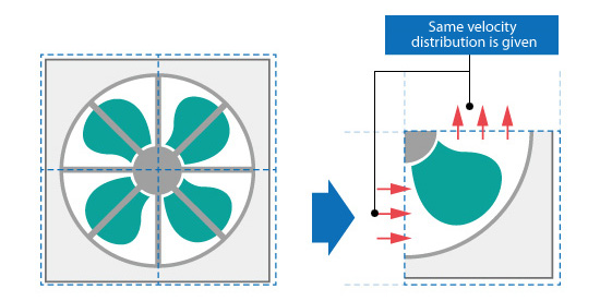
Figure 5.18: Example of a periodic boundary condition
To perform an analysis properly, selecting the appropriate boundary condition is critical. If an improper boundary condition is assigned, the physical phenomena will not be properly simulated, resulting in erroneous results. Moreover, the calculation may also be unstable.
5.6 Initial condition
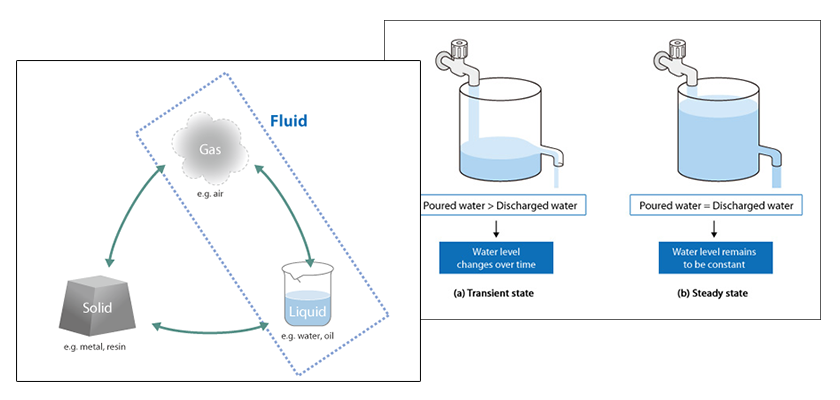
The condition that defines the initial state of an analysis is called an initial condition. For example, if the ambient temperature at the start of an analysis is 25°C, this is its initial state. “Temperature: 25°C” is set as an initial condition.
The initial condition is important particularly for a transient analysis. Figure 5.19 shows an environment at 20° C with two objects, whose temperatures are 50° C and 100° C, respectively placed in the environment. The object temperatures at the initial state are different. The temperatures are also different after five minutes as shown in the figure. Different initial conditions will make the calculation progress differently in a transient analysis.
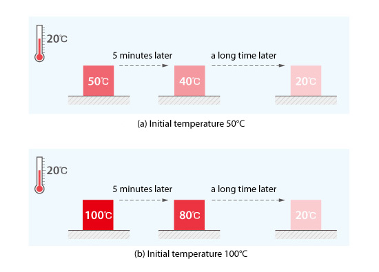
Figure 5.19: Initial temperature and time variation of temperature
However, in both cases shown in Figure 5.19, the object temperature will be 20°C after a sufficient time. This is the same temperature as that of the surrounding space. This is the temperature that would be achieved for a steady-state analysis. The initial condition does not affect the calculation results for a steady-state analysis.
The same can be said of other variables besides temperature. If the calculated results are different for two steady-state analyses with different initial conditions, either or both of the calculations may not have reached steady state yet.
Note that the calculation time will be reduced for a steady-state analysis by setting the initial conditions, for each cell where parameter values are calculated, close to the anticipated steady state solution values.

About the Author
Atsushi Ueyama | Born in September 1983, Hyogo, Japan
He has a Doctor of Philosophy in Engineering from Osaka University. His doctoral research focused on numerical method for fluid-solid interaction problem. He is a consulting engineer at Software Cradle and provides technical support to Cradle customers. He is also an active lecturer at Cradle seminars and training courses.

