5.3 Computational domain

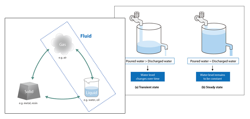
Let's think about analyzing the air flow around an airplane in flight. To analyze the real flow perfectly, unlimited space would be needed because the space around the airplane consists of the sky and then outer space. Unfortunately, the computer must process a finite number of values.
Therefore, an appropriate and finite analysis space or area must be defined around the airplane and this space is called the analysis domain.

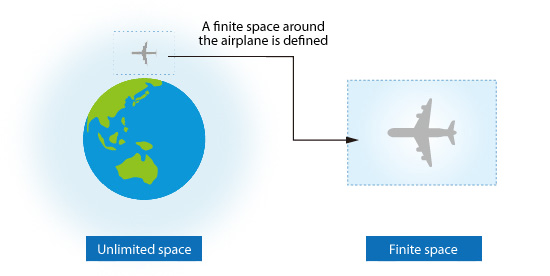
Figure 5.9: Computational domain

The faces of the computational domain are not solid walls, and they are created just to define a physical boundary for the calculation. Therefore, the computational domain must be large enough so that its faces are sufficiently far from the target object to prevent the faces of the computational domain from artificially influencing the flow over the object. For example, when some of the flow is outside the computational domain and flows back into the computational domain as shown in the lower right part of Figure 5.10 (a Bad example of defining the boundaries of the domain), the flows shown by the dotted lines are not correctly simulated. Consequently, the calculated result will likely be different from the real result. On the other hand, while it may seem simpler to select a very large domain, specifying an unnecessarily large domain will require much more time to obtain the solution.

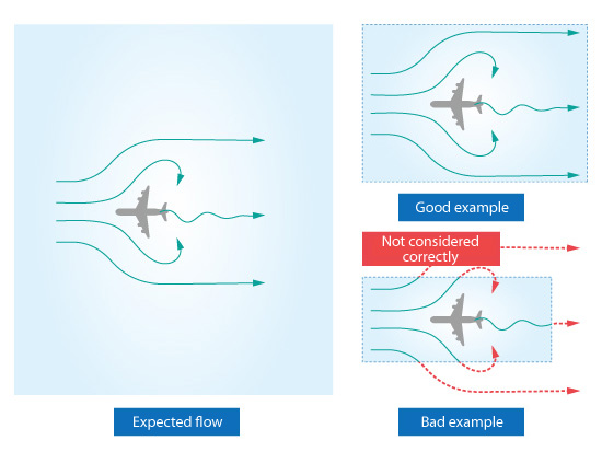
Figure 5.10: Creating a computational domain

Determining the appropriate size of a computational domain can be challenging but becomes easier as the analyst gains more experience and an increased understanding of how flows behave.

5.4 Division of a space

The relationship between flow variables in neighboring spaces is calculated by discretizing the equations (e.g. momentum, energy, and continuity equations). Discretizing requires dividing the computational domain into many tiny spaces where each space is called an element or cell . The equations are expressed as functions of the geometrical relationships between adjacent cells. A set of elements or cells is called a mesh or grid .
Parameters, such as fluid velocity and temperature , are calculated for each element, and each element has one value for each parameter. The value of the parameter is constant within the entire element. Hence, resolution is improved as the elements become smaller. Figure 5.11 is an example of an analysis result where the temperature is high at the center of the model and low at its periphery. The figure shows that the larger the elements are, the larger the range can be for the parameter in the element (maximum – minimum value within the element). In other words, the parameter distribution will be coarser as the element size increases.

Figure 5.11: Element size and the analysis result

In general, the calculation requires less time for larger elements (fewer total elements) because fewer calculations must be performed. However, the calculation result will be less accurate due to the coarser distribution of the parameters. In contrast, the calculation will require more time for smaller elements (more total elements because more calculations must be performed. However, the calculation result will be more accurate and provide better resolution.

In many cases, a finer mesh is generated around the selected features in the model where the flow and temperature vary rapidly (large gradients). On the other hand, a coarser mesh can be used where flow and temperature vary slowly.
There are two meshing methods as shown in Figure 5.12. Elements are placed in a repeatable pattern in a structured mesh (left) and irregularly in an x /dcms_media/image/en_column_basic_unstructured mesh   (right).

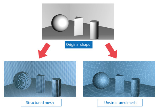
Figure 5.12: Mesh generation

Figure 5.13 shows the element types most generally used in each meshing method.

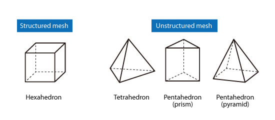
Figure 5.13: Typical element types

In a 3D analysis, the structured mesh elements are hexahedrons, and they are placed in a repeatable pattern. This mesh is easily generated and the calculation speed is very fast. On the other hand, an unstructured mesh uses tetrahedrons and pentahedrons shaped elements. Mesh generation is more challenging compared to a structured mesh; however, the elements can be placed much more freely. Therefore, unstructured mesh is suitable for representing complicated geometries.

---

About the Author
Atsushi Ueyama | Born in September 1983, Hyogo, Japan 

He has a Doctor of Philosophy in Engineering from Osaka University. His doctoral research focused on numerical method for fluid-solid interaction problem. He is a consulting engineer at Software Cradle and provides technical support to Cradle customers. He is also an active lecturer at Cradle seminars and training courses.