5.8 Progress of time

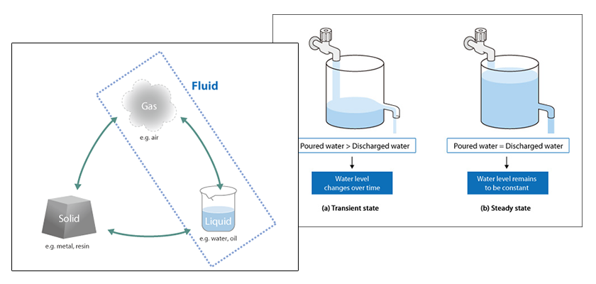
There are two types of analyses: a steady-state analysis and a transient analysis.
In a steady-state analysis, only the final state is obtained without any change over time. In fact, time does not have any meaning in a steady-state analysis. Because of this, the states before the calculation reaches the final state do not have any physical significance. This is all another way of saying that only the final state has meaning in a steady-state analysis.
On the other hand, in a transient analysis, the analysis is separated by short time intervals. The state of a phenomenon from one moment to the next is calculated and the procedure is repeated. The states for each calculation step are determined, and represent the physical conditions at that particular instant in time. The change in state can be calculated until the phenomenon reaches the final state.
Time step is the time from one moment to the next. For a transient analysis with a constant time step, a larger time step can decrease the number of calculation iterations and lead the calculation to reach the final solution more quickly. However, the prediction accuracy degrades. Therefore, determining an appropriate time step is crucial in a transient analysis.

Courant number is a parameter used for determining the time step and is defined by the following equation:

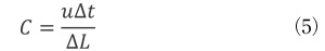
where,

C: Courant number
u: Velocity
Δt: Time step
ΔL: Element width.

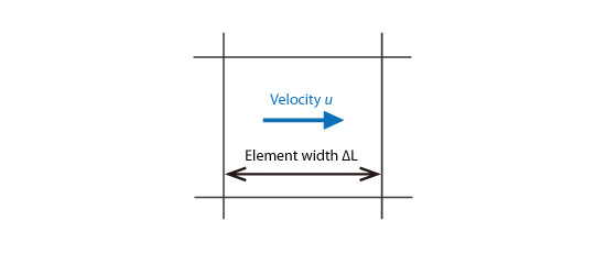
Figure 5.21: Parameters for Courant number

The Courant number relates the number of elements which the flow passes through in one time step.
For example, when the Courant number is 1, the flow at a certain point moves into the neighboring element in one time step as shown in the upper part of Figure 5.22. Good accuracy can be obtained when the Courant number is 1.
On the other hand, if the Courant number is 10, the flow passes through 10 elements in one time step as shown in the lower part of Figure 5.22. Since the flow passes this far in one time step, this is equivalent to having a 10 times coarser mesh with the Courant number = 1.

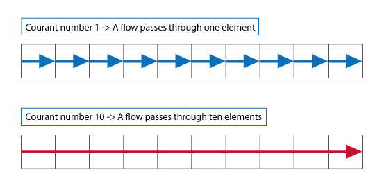
Figure 5.22 Flow difference depending on Courant number

The Courant number is determined as a function of the size of each element and the velocity through the element. The Courant number becomes larger when the flow passes through elements with small widths. Likewise, the Courant number increases when the flow passes through constant width elements with a higher velocity. Often times, the element-width and velocity will be different depending on where the element is located in the model. Therefore, the Courant number also differs depending on location. In consideration of the time needed for analysis, the time interval should be set so that the maximum Courant number is as small as possible.
 

About the Author
Atsushi Ueyama | Born in September 1983, Hyogo, Japan  

He has a Doctor of Philosophy in Engineering from Osaka University. His doctoral research focused on numerical method for fluid-solid interaction problem. He is a consulting engineer at Software Cradle and provides technical support to Cradle customers. He is also an active lecturer at Cradle seminars and training courses.