Chapter 3 Basics of Flow V

3.2.4 Laminar flow and turbulent flow

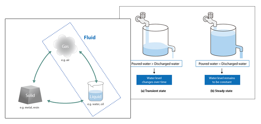
A flow has two states: laminar and turbulent. A fluid flow with regular, predictable motion is called laminar flow. On the other hand, a flow with irregular, unpredictable motion is called turbulent flow.

Consider water running from a tap to illustrate the two states. When the tap is turned on just a small amount, water flows straight down in a very well-behaved and predictable stream as shown in (a) of Figure 3.15. The more the flow increases the more turbulent the water flow becomes. The surface of the water creates waves as shown in (b).

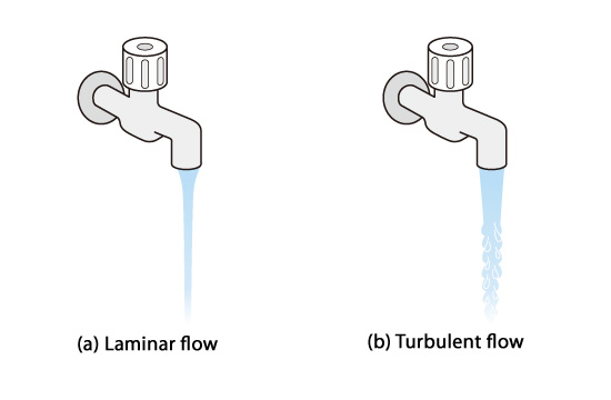
Figure 3.15: Water running from a tap

In 1883, a British scientist named Osborne Reynolds (1842-1912) classified flows as either laminar or turbulent from a series of experiments known as the Reynolds’ experiment. In the experiment, flows were visualized by pouring a stream of ink into a pipe in which water flows. The result showed that, when the water velocity was low, the ink moved downstream in a continuous straight line as shown in (a) of Figure 3.16. In this case, the flow was laminar. However, when the water velocity was high, the ink started in a straight line but began oscillating and quickly dispersed throughout the pipe. This flow was turbulent.

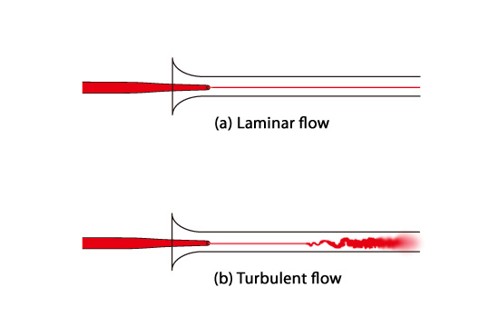
Figure 3.16: Reynolds’ experiment

In the experiment, Reynolds discovered a dimensionless number could be used to classify flows as either laminar or turbulent. This number is called the Reynolds number. The Reynolds number Re is defined by the following equation:

where,

L: Characteristic length
       (In this example, L is the inside diameter of the pipe)
U: Representative velocity
       (Here, it is the average velocity of the flow passing through a cross-section of the pipe)
ρ : Fluid density
μ: Viscosity coefficient

The denominator of the equation expresses the viscous force of the fluid. The numerator of the equation expresses the inertial force. Hence, the Reynolds number is the ratio of the inertial force to the viscous force. When two flows are geometrically similar and have the same Reynolds number, this means their ratio between their inertial forces and their viscous forces will be the same. Thus, the behavior of the two flows will be essentially the same. This law is called the Reynolds' law of similarity.

Consider another example. Suppose you want to simulate the air flow around an automobile moving at a speed of 50 km/h by using a half-size model in a wind tunnel as shown in Figure 3.17. The equation for the Reynolds number says the air velocity should be 100 km/h since the characteristic length has been cut in half to maintain a constant Reynolds number.

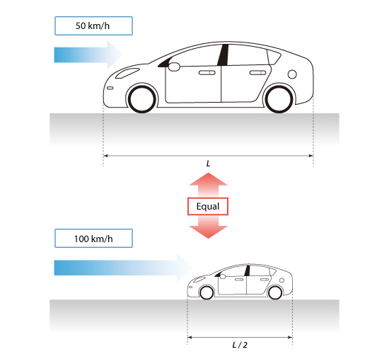
Figure 3.17: Reynolds' law of similarity

A closer look at the Reynolds number reveals the following: When the fluid viscosity is large or the fluid velocity is low, the viscous force becomes dominant. When this occurs, the Reynolds number will be small and the fluid flow will be laminar. On the other hand, when the fluid viscosity is small or the velocity is high, the inertial force becomes dominant. Thus, the Reynolds number of the fluid will be large and the fluid flow will be turbulent.

The range of Reynolds number for the transition from laminar to turbulent flow in a pipe is generally 2,000 to 4,000. These values are just approximated and the actual values will vary depending on the state or conditions of the flow.

In this final example, we can determine whether the air flow around a bicyclist is laminar or turbulent. Figure 3.18 shows the air flow around a bicyclist traveling at 14.4 km/h.

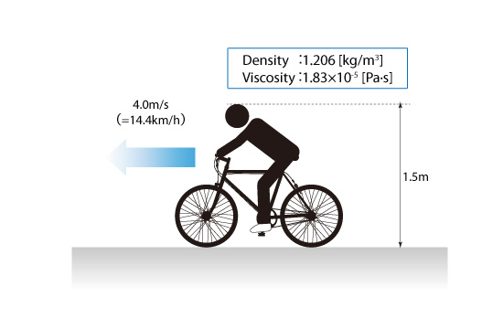
Figure 3.18: Person riding on a bicycle

The Reynolds number is calculated using the following equation for the flow of air.

The calculated value for the Reynolds number is 400,000, far greater than the aforementioned approximate value of 2,000 - 4,000 denoting the conditions when the flow transitions from laminar to turbulent. We find that the majority of flows observed in our daily lives is turbulent.

A turbulent flow can be either an advantage or disadvantage. A turbulent flow increases the amount of air resistance and noise; however, a turbulent flow also accelerates heat conduction and thermal mixing. Therefore, understanding, handling, and controlling turbulent flows can be crucial for successful product design.

---

About the Author
Atsushi Ueyama | Born in September 1983, Hyogo, Japan 

He has a Doctor of Philosophy in Engineering from Osaka University. His doctoral research focused on numerical method for fluid-solid interaction problem. He is a consulting engineer at Software Cradle and provides technical support to Cradle customers. He is also an active lecturer at Cradle seminars and training courses.