Search for a shape with minimum fluid drag (4)

In the previous column, we searched for a shape with which drag force becomes the minimum with the Reynolds number 650. In this column, we search for a shape with which drag force becomes the minimum with the Reynolds number 650,000.

In the same way as in the previous column, drag coefficient is obtained by performing a CFD analysis using a model created based on design of experiments with EOopti. The cross section area ratio in the previous column is used considering the similarity. The result is input to EOopti, and the optimization is executed to obtain response surfaces and optimal solution distribution. Figure 4.1 shows the response surface of cross section area ratio, which is the same result as in the previous column because of the similarity. Figure 4.2 shows the response surface of drag coefficient. The drag coefficient increases steeply from around Y=30%. In addition, it is found that X coordinate of the intermediate point is negative when Y coordinate is 30% or smaller; that is, drag coefficient is small when the intermediate point is located toward upstream.

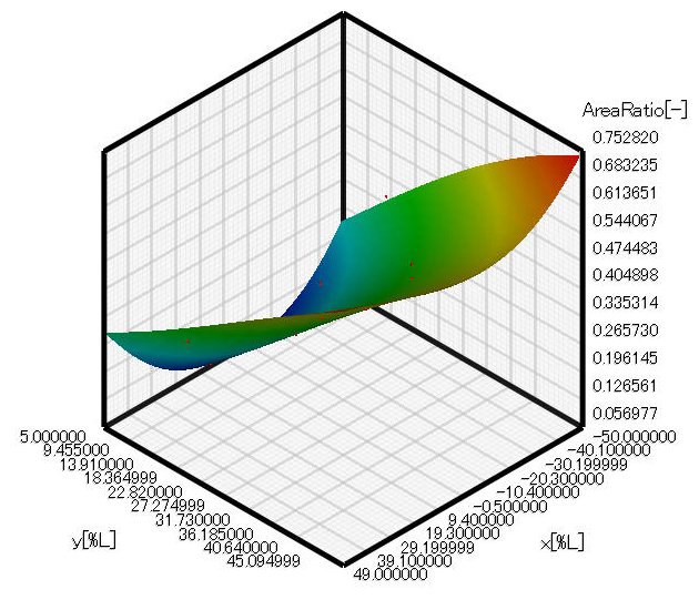
Figure 4.1 Response surface of cross section area ratio

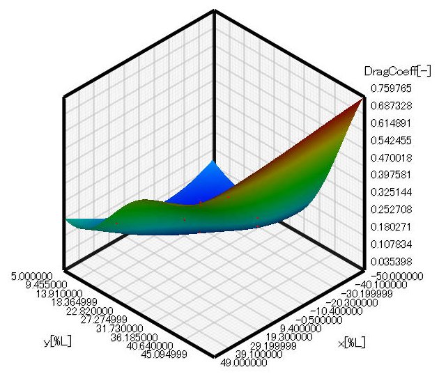
Figure 4.2 Response surface of drag coefficient

Figure 4.3 shows the distribution of optimal solutions. The closer to the bottom right corner of the graph it is, the larger the cross section area ratio is and the smaller the drag coefficient is, which is the optimal solution. The red circle in the graph indicates the cross section area ratio and drag coefficient of a cylinder. In the graph, we can see that drag coefficient increases steeply when the cross section area ratio exceeds 0.55. In figure 4.4, the worst solutions (shown in red circles), i.e., the ones with small cross section area ratio and large drag coefficient, are added to Figure 4.3. In this graph, we find that there is a factor of five or larger difference in drag coefficient between the optimal and worst solutions for the same cross section area ratios. In the previous column with the Reynolds number 650, the difference in drag coefficient between the optimal and worst solutions is only by a factor of about 1.7. Compared to this, it is shown that the shape has a greater influence on drag coefficient in the high-Reynolds-number regime.

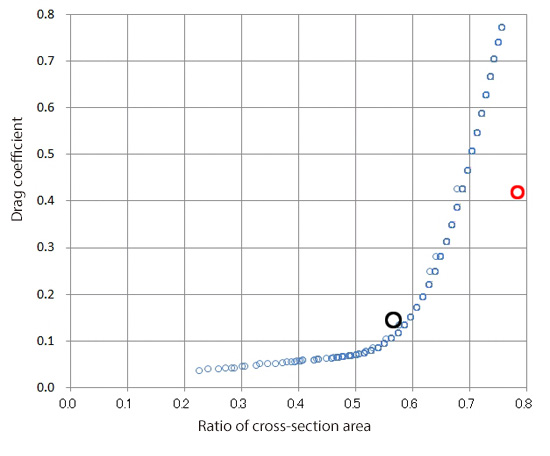
Figure 4.3 Optimal solution distribution

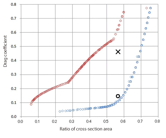
Figure 4.4 Comparison of optimal and worst solution distributions

To find the shape with which solutions become optimal, X and Y coordinates of the intermediate point of the optimal solutions are plotted (Figure 4.5). The blue circles in the figure indicate the locations of the intermediate point of the optimal solutions, while red circles indicate those of the worst solutions. In the graph, we observe that the optimal solutions are the ones with negative X coordinates of the intermediate point, which means the shapes with fatter upstream portions; on the other hand, the worst solutions are those with positive X coordinates of the intermediate point, which means the shapes with fatter downstream portions. A proposed optimal shape, therefore, is the one with X=−45% and Y=25%, as it is drawn in Figure 4.6. In contrast, a proposed worst shape is the one with X=45% and Y=25%, which is the optimal shape flipped in the streamwise direction. Models for the proposed optimal and worst shapes are created and analyzed using SC/Tetra to obtain drag coefficient.

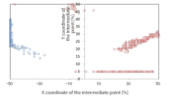
Figure 4.5 Position of the intermediate point to give optimal solutions

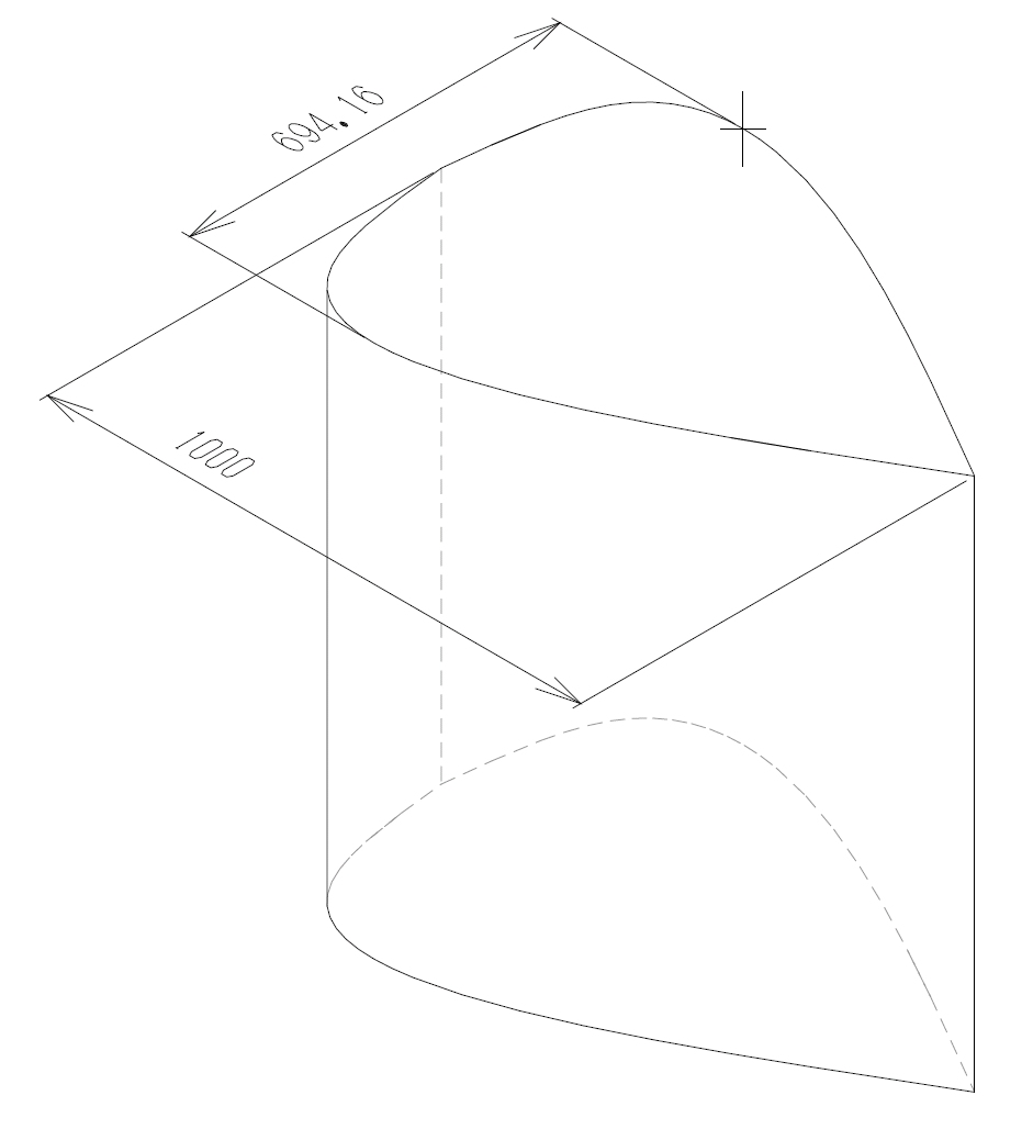
Figure 4.6 Proposal of optimal shape

The cross section area ratio and drag coefficient of the optimal shape is drawn in Figure 4.4 with a black circle. The worst shape is also drawn in Figure 4.4 with a × sign. Drag coefficient of the worst shape is roughly three times larger than that of the optimal shape. The optimal and worst shapes are mirror images of each other, and their cross sectional areas are the same. Drag force on the worst shape, therefore, is also roughly three times larger than that on the optimal shape. Since drag force is proportional to the square of velocity, if the cross section area ratio and the force required to move against the flow are proportional, the optimal shape can move √3≈1.7 times as fast as the worst shape. Figures 4.7, 4.8, 4.9, and 4.10 show pressure contour of the optimal shape, velocity distribution for the optimal shape, pressure contour of the worst shape, and velocity distribution for the worst shape, respectively. Comparing the pressure contours in Figure 4.7 and 4.9, we can see that a negative pressure region exists behind the worst shape object, which increases the drag force. By comparing the velocity distributions in Figure 4.8 and 4.10, the large vortex behind the worst shape object can be considered a possible cause of the pressure drop and the existence of the negative pressure region.

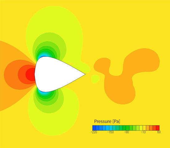
Figure 4.7 Pressure distribution for the proposed optimal shape

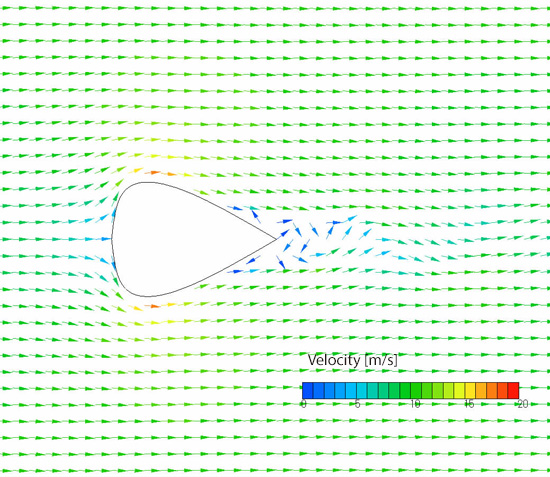
Figure 4.8 Velocity distribution for the proposed optimal shape

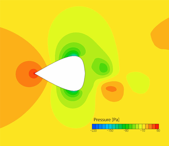
Figure 4.9 Pressure distribution for the proposed worst shape

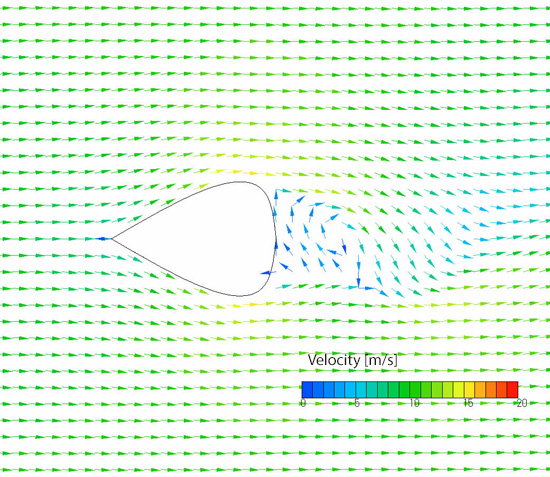
Figure 4.10 Velocity distribution for the proposed worst shape

The next column will discuss why optimal solutions are different depending on the Reynolds number.

[Reference] Kikaikougaku binran ‘Ryutai kougaku’ (Mechanical engineering handbook, ‘Fluid engineering’),
User's Guide Optimization (Option)

---

About the Author 
Professor Gaku Minorikawa | Faculty of Science and Engineering, 
Department of Mechanical Engineering, Hosei University
Certified environmental measurer (noise and vibration)

• 1992 Joined EBARA CORPORATION
• 1999 Became an assistant at Hosei University Faculty of Engineering
• 2001 Obtained Doctor of Engineering at Tokyo Institute of Technology
• 2004 Became Assistant Professor at Hosei University Faculty of Engineering
• 2010 Became Professor at Hosei University Faculty of Science and Engineering

About the Author 
Takahiro Ito | Senior Researcher, ORIENTAL MOTOR Co., Ltd.

• 1982 Graduated University of Tsukuba (College of Engineering Sciences) and joined Nippon Steel Corporation, where he worked on the development of heating and cooling facilities.
• 1988 Joined ORIENTAL MOTOR Co., Ltd. and worked on the design and development of ventilator vanes and frames.
• 2008 Obtained Doctor of Engineering at Hosei University.
• He is Senior Researcher of ORIENTAL MOTOR Co., Ltd. (as of January 2014).