
Case Study – Learn about Thermo-Fluid Analyses Optimization No. 5: Search for a shape with minimum fluid drag (2)
Search for a shape with minimum fluid drag (2)
The previous column described how to obtain an arbitrary shape with which a cross section is the maximum and the drag coefficient is the minimum, as a method to search for a shape with which fluid resistance is the minimum.
In this column, we create the model. Before the creation, we will examine velocity and representative length.
When a fluid is air at 20º C, its kinematic viscosity coefficient is 1.54 x 10⁻⁵ m2 /s. When the representative length is 10 mm and velocity is 1 m/s, Reynolds number (Re) is 650, which is small. The analysis with the Reynolds number of 650 simulates a flying insect. On the other hand, when the representative length is 1 m and velocity is 10 m/s, Reynolds number is 650,000, which is large. The analysis with the Reynolds number of 650,000 simulates a large-size model airplane flying at a velocity of 40 km/h.
First of all, perform an analysis with a cylinder model to check the analysis field. The coordinate conversion of SC/Tetra is used to change the model size. Create a medium-size model, i.e., the representative length is 100 mm. Then, as the entire flow field region, create an enclosure whose upstream and downstream lengths and widths are ten times as long as the representative length. (See Figure 2.1) The height is set to 100 mm. This is the value that SC/Tetra recognizes the analysis as two-dimensional. Create the model with CAD and load the obtained 3D shape in SC/Tetra. Then, define INLET, SURFACE, and OUTLET as boundary conditions. (See Figure 2.1) Save them as a model. When Re = 650, scale down the model to one-tenth and set a boundary condition of INLET to 1 m/s of velocity. On the other hand, when Re = 650,000, scale up the model by a factor of ten and set a boundary condition of INLET to 10 m/s of velocity.
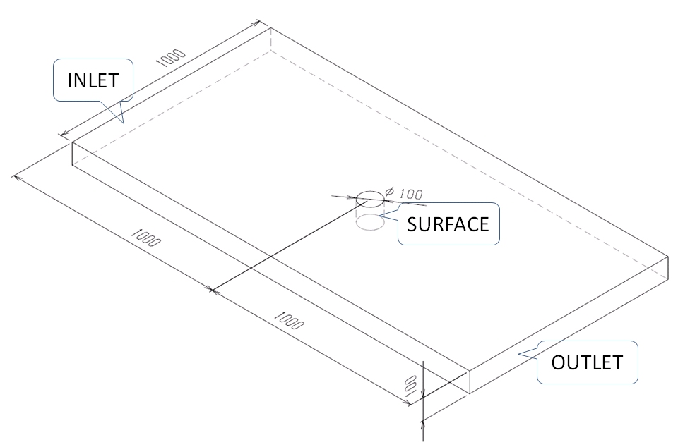
Figure 2.1: Shape of CAD model
Perform the calculation as a two-dimensional analysis using Adaptive Mesh Refinement method with these conditions. The results are shown in Figure 2.2 and 2.3. Figure 2.2 is a velocity distribution map with Re = 650 while Figure 2.3 is the map with Re = 650,000. Drag coefficient (CD) when Re = 650 is 1.22 while it is 0.42 when Re = 650,000. The results almost agree with the data in JSME (The Japan Society of Mechanical Engineers) Mechanical Engineers' Handbook (only in Japanese) and appropriate for an analysis. Then, change the name of the condition setting file (S file) and model name. Use them in the analysis setting of the cylinder whose cross section has an arbitrary shape. You can increase the work efficiency and avoid input errors by the name change.
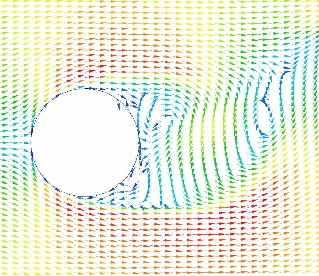
Figure 2.2: Velocity distribution when Re = 650
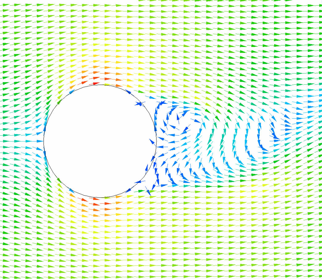
Figure 2.3: Velocity distribution when Re = 650,000
Next, create a cylinder model whose cross section has an arbitrary shape. Design variables are X and Y coordinates of an intermediate point (two variables). Therefore, the number of samples is (2 + 1)·(2 + 2) = 12. X coordinate ranges from −50 to 50 and Y coordinate from 10 to 50. Optimal solutions are searched for with EOopti. The procedure is done in the dialog shown in Figure 2.4.
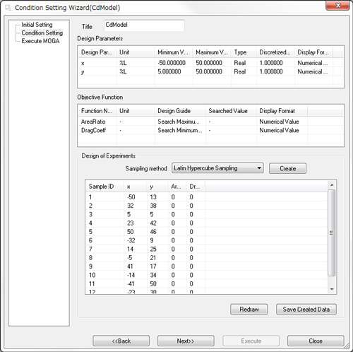
Figure 2.4: Condition setting in EOopti
Save the values in CSV format. Then, draw a spline curve with the intermediate point whose X and Y coordinates have been designed above, and create a CAD model. Calculate cross-section area and its ratio to the area of a square. This is the objective function AreaRatio shown in Figure 2.4. Next, create a model with SC/Tetra and prepare models and S files for Re = 650 and 650,000 in the same manner as that of the cylinder calculation. Then, perform an analysis using Adaptive Mesh Refinement method. Calculate drag coefficient from the obtained result. This is the objective function DragCoeff in Figure 2.4. Repeat the procedure as many times as the number of samples and input the obtained result in an appropriate space in the dialog (Figure 2.4).
The next column will explain about optimal solutions when Reynolds number is 650.
[Reference] Kikaikougaku binran ‘Ryutai kougaku’ (Mechanical engineering handbook, ‘Fluid engineering’),
User's Guide Optimization (Option)

About the Author
Professor Gaku Minorikawa | Faculty of Science and Engineering,
Department of Mechanical Engineering, Hosei University
Certified environmental measurer (noise and vibration)
- 1992 Joined EBARA CORPORATION
- 1999 Became an assistant at Hosei University Faculty of Engineering
- 2001 Obtained Doctor of Engineering at Tokyo Institute of Technology
- 2004 Became Assistant Professor at Hosei University Faculty of Engineering
- 2010 Became Professor at Hosei University Faculty of Science and Engineering

About the Author
Takahiro Ito | Senior Researcher, ORIENTAL MOTOR Co., Ltd.
- 1982 Graduated University of Tsukuba (College of Engineering Sciences) and joined Nippon Steel Corporation, where he worked on the development of heating and cooling facilities.
- 1988 Joined ORIENTAL MOTOR Co., Ltd. and worked on the design and development of ventilator vanes and frames.
- 2008 Obtained Doctor of Engineering at Hosei University.
- He is Senior Researcher of ORIENTAL MOTOR Co., Ltd. (as of January 2014).

