Shape optimization for a can (3)

In EOopti, the user must determine the number of samples. The reference number is greater thanwhere N denotes the number of design variables. However, the reference numbermay not be enough samples for complicated phenomena. How many samples are necessary for such phenomena? We can use a simple function to show how the shape of response surfaces and optimal solutions change depending on the numbers of samples.

Function used for the experiment

As an example, we will search for the maximum value of the function cos(x) + cos(y) in the range . The shape of the function is shown in Figure 3.1 and has multiple maximum values. In the range , the function is a maximum when x = 0, y = 0. The maximum value is 2.

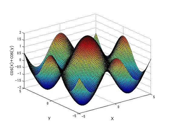
Figure 3.1: cos(x) + cos(y)

This function has two independent variables, x and y; therefore, the minimum number of recommended samples will be (2+1)·(2+2) = 12. We will use EOopti to perform the optimization for sample sizes of 12, 24, and 36. We will check the shape of the response surfaces and the optimal solutions for each case.

Figure 3.2 shows the response surface for 12 samples. The symmetry with the center at x = 0, y = 0 is lost. In addition, the maximum value is approximately 1.56.

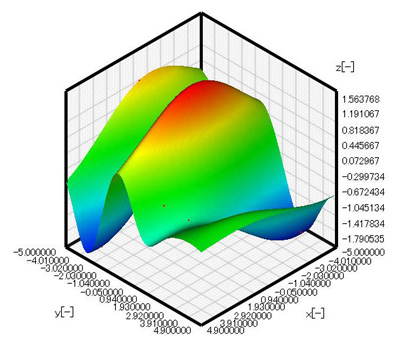
Figure 3.2: Response surface for 12samples

Figure 3.3 shows the response surface for 24 samples. Symmetry is improved compared with Figure 3.2; however, the response surface is asymmetric about y = 0. The response surface shape will also differ depending on the allocation of sampling points so the solution results may not be the same. Figure 3.4 shows the response surface for 36 samples. The shape of the response surface is the same as shown in Figure 3.1. In addition, the maximum value is also 2 which agrees with the analysis result.

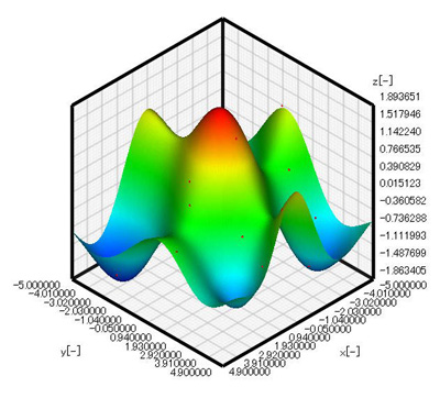
Figure 3.3: Response surface for 24 samples

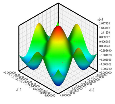
Figure 3.4: Response surface for 36 samples

The next assessment is for the location of the indicated maximum value for the three different sample sizes and their magnitudes. Figure 3.5 shows the x and y coordinates where the value of the response surface is the maximum. The x coordinate is on the horizontal axis, and y is on the vertical axis. For 12 samples, the maximum value of the response surface occurs at x = -0.19 and y = -0.73. For 24 samples, the response surface maximum occurs at x = -0.22 and y = -0.06. When 36 samples are used, the response surface maximum occurs at x = -0.0002 and y = -0.0031. The maximum value is also 2.0. This result agrees very well with the analytically obtained result, i.e., x = 0 and y = 0, and the maximum value is 2.

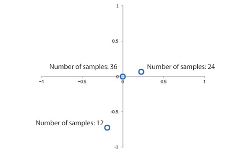
Figure 3.5: Location of optimal solutions depending on the number of samples

Efficient Global Optimization (EGO) can be used to locally improve the shape of the response surface around the optimal solution (compared to improving the shape of the entire response surface). EGO enables the user to improve the shape of the response surface by only adding small number of samples. The Expected Improvement (EI) parameter in EOopti can be used instead of an objective function to search for optimal solution. EI indicates the degree that new samples will be the minimum/maximum values when they are added to the current samples. By adding pairs of the design parameter and objective function where EI will be the maximum, and then using EOopti to search for optimal solutions of EI, a new local maximum can be identified. Performing the search four additional times generates the response surface shown in Figure 3.6. While this response surface is not as good as the response surface for 24 samples shown in Figure 3.3, the position of the optimal solution is x = 0.025 and y = -0.108, and the maximum value is 1.98 (Figure 3.7). With only 16 samples, we have obtained a solution that nearly matches the precision of a response surface generated using 36 samples.

For details about the addition of the number of samples and precision improvement using EI, please refer to the help file in EOopti.

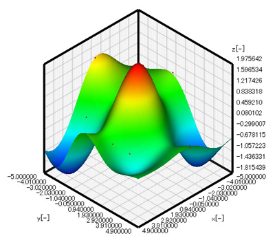
Figure 3.6: Add four samples with which EI will be the maximum to the result of the number of samples 12

Figure 3.7: Difference of optimal solutions depending on the number of samples

In the next article, the shape for the lowest fluid resistance and the largest cross-sectional area will be obtained using SC/Tetra and EOopti.

(Reference) User's Guide Optimization (Option)

---

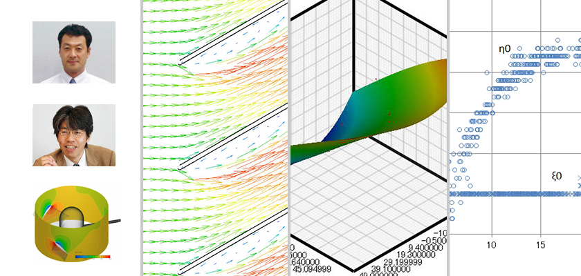
About the Author 
Professor Gaku Minorikawa | Faculty of Science and Engineering, 
Department of Mechanical Engineering, Hosei University
Certified environmental measurer (noise and vibration)

• 1992 Joined EBARA CORPORATION
• 1999 Became an assistant at Hosei University Faculty of Engineering
• 2001 Obtained Doctor of Engineering at Tokyo Institute of Technology
• 2004 Became Assistant Professor at Hosei University Faculty of Engineering
• 2010 Became Professor at Hosei University Faculty of Science and Engineering

About the Author 
Takahiro Ito | Senior Researcher, ORIENTAL MOTOR Co., Ltd.

• 1982 Graduated University of Tsukuba (College of Engineering Sciences) and joined Nippon Steel Corporation, where he worked on the development of heating and cooling facilities.
• 1988 Joined ORIENTAL MOTOR Co., Ltd. and worked on the design and development of ventilator vanes and frames.
• 2008 Obtained Doctor of Engineering at Hosei University.
• He is Senior Researcher of ORIENTAL MOTOR Co., Ltd. (as of January 2014).