Shape optimization for a can (2)

In the previous article, the shape of a can was optimized by deriving the conditions which minimize the surface area and joint length of the can for fixed volume. This problem can be easily solved by transforming the equation which expresses the length of the edge, volume, and surface area of a cylinder. However, a real phenomenon can rarely be expressed by a single equation. To obtain a combination of optimal solutions for a complicated phenomenon, optimization software can be used. Here, the EOopti optimization tool will be used to optimize the shape of a can.

Review of the problem and optimization procedure

First, we'll review the problem again. Then, we will outline the procedure for solving the problem.
To optimize the shape of a 1,000 cm3 cylindrical can (Figure 2.1), the ratio of the can's height to diameter which produces the minimum surface area and joint length must be calculated.

Figure 2.1: Shape of a can

Figure 2.2 shows the optimization work flow for the EOopti optimization tool. First, perform Design of Experiments (DOE). In this example, specify several pairs of heights and diameters. Next, obtain the results from the experiment or CAE calculation using the parameters defined in DOE. For this example, a software program such as Microsoft^® Excel^® can be used to calculate the surface area and joint length of the can from the height to diameter ratio. Some commercial optimization tools can perform the entire sequence of discrete calculations for the analysis, including CAE calculations. These tools will also check the calculation results to judge optimality, and perform a second CAE calculation for the new proposed conditions. However, to fully automate optimization, the combination of hardware and software performance must be capable of automatically processing the optimization and modeling activities. To do this, an approximation formula is obtained from the CAE calculation results, and this formula is used for the general optimization. The approximation formula corresponds to the response surface formula block shown in Figure 2.2. EOopti uses the response surface formula to search for an optimal solution.

Figure 2.2: Optimization workflow

Optimization using EOopti

First, select several sets of design parameters. This process is called sampling.
Calculate the number of sample sets based on the formulawhere n indicates the number of design parameters.
The number of sample sets should be the calculated value or greater. For example, for regression using quadratic equations of n variables, the following number of terms will be required:
Constant: 1, Linear: n, Quadratic: n, Product between variables:
To set each term, at a minimum, the same number of sets of variables as terms is required. In total, the required number of sample sets of variables will be.
To reduce the uncertainty of the samples, the doubled number ofis generally used, which is. The number of sample setsis a reference number for regression using quadratic equations. Thus, for more complicated phenomena, samples must be added according to the analysis results. Furthermore, the number of samples generally will be the second power of the design parameters; therefore, an extremely large number of design parameters should be avoided.

In this example, the design parameter is only H/D, and the number of samples will be
(1 + 1) · (1 + 2) = 6. However, 12 samples will be used because EOopti does not permit using less than 7 samples. After inputting the number of samples, click the Create button in the dialog shown in Figure 2.3 to create an optimal combination of experimental conditions. Next, execute a CFD analysis according to the created combination. Then input the result, and click Next button. Upon doing this, the dialog shown in Figure 2.4 appears.

In the dialog, set the options as necessary and click the Execute button. Then, EOopti creates a response surface equation according to the input values and performs the optimization calculation based on the equation.

Figure 2.3: Dialog to input the experiment plan and the analysis result

Figure 2.4: Dialog for the response surface calculation and the search for the optimal solution

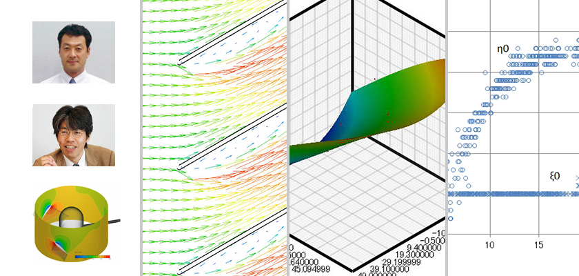
After the optimization calculation, the response surface can be displayed in 3D. The contribution of the design parameters to the objective variables and the distribution of optimal solutions can also be displayed. Figure 2.5 shows the distribution of optimal solutions. This is the result option that is used most often. In Figure 2.5, the horizontal axis indicates the surface area, and the vertical axis indicates the joint length. Both values are obtained for a certain ratio of the height to the diameter of the can. By clicking a point anywhere in the figure, the design parameters and objective variables at this point are displayed as shown in Figure 2.5. Showing these values to the product design team, manufacturing, purchasing, and sales, data is provided to evaluate proposed designs more objectively. This is the visualization of design process.

Figure 2.5: Distribution of optimal solutions

EOopti outputs the analysis result in a CSV file. Figure 2.6 shows the comparison between the analysis result and the calculated result from the previous article. The red circles in the figure indicate the optimal solutions calculated by EOopti. They agree well with the solid curve where the curve indicates the result obtained by transforming the equation of the surface area and the joint length. The following optimal solutions can be obtained:
- The surface area is smallest when the height and the diameter are equal.
- The joint length is shortest when the height is approximately 3.1 times longer than the diameter.

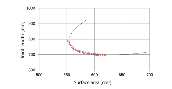
Figure 2.6: Comparison of the result of EOopti with that obtained by using equations

When using EOopti, the first thing to determine is the number of samples. The number of samples should be greater than the value obtained by the formulawhere the number of design parameters is n. However, the number of samples will also depend on the shape of the response surface. In the next article, we will see how the response surface changes as the number of samples changes. We will also see how the optimal solutions can be obtained by using simple functions.

(Reference) User's Guide Optimization (Option)

---

About the Author 
Professor Gaku Minorikawa | Faculty of Science and Engineering, 
Department of Mechanical Engineering, Hosei University
Certified environmental measurer (noise and vibration)

• 1992 Joined EBARA CORPORATION
• 1999 Became an assistant at Hosei University Faculty of Engineering
• 2001 Obtained Doctor of Engineering at Tokyo Institute of Technology
• 2004 Became Assistant Professor at Hosei University Faculty of Engineering
• 2010 Became Professor at Hosei University Faculty of Science and Engineering

About the Author 
Takahiro Ito | Senior Researcher, ORIENTAL MOTOR Co., Ltd.

• 1982 Graduated University of Tsukuba (College of Engineering Sciences) and joined Nippon Steel Corporation, where he worked on the development of heating and cooling facilities.
• 1988 Joined ORIENTAL MOTOR Co., Ltd. and worked on the design and development of ventilator vanes and frames.
• 2008 Obtained Doctor of Engineering at Hosei University.
• He is Senior Researcher of ORIENTAL MOTOR Co., Ltd. (as of January 2014).