Methods of turbulent flow calculation (4)
Wall condition of RANS (Reynolds-Averaged Navier-Stokes) model

10.1: Wall condition of RANS model

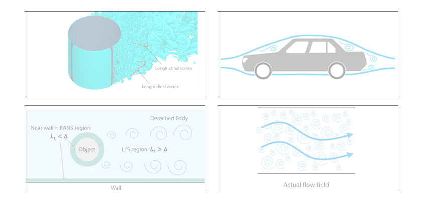
We have discussed that RANS model is aimed at calculating averaged flow fields and that it incorporates the effect of unsteady vortex motions by eddy viscosity. Another important topic for RANS model is how to deal with walls. In this column, we will discuss wall conditions in RANS model.

On walls, flows are stationary. Farther away from walls, they become faster. You may understand this easily if you think about the flow of a river. You would agree with my impression that the flow away from riverbanks is faster (and more dangerous) than the flow near banks. In a turbulent flow, this change in velocity according to the distance from wall becomes sharper. The reason for the sharp change may be understood with an idea that the flow is strong (has a large momentum) and therefore it is fast until very close to the walls. In a flow calculation, this change in velocity must be captured accurately; however, since the distance in which this change occurs is very short compared to the size of the entire flow field, arranging mesh based on this distance can lead to an enormous scale of calculation (Figure 10.1). Ingenuity, therefore, is needed for enabling a calculation with thicker mesh near walls.

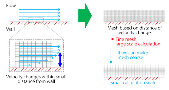
Figure 10.1: Mesh near walls and scale of calculation

10.2: Wall function

Ingenuity for enabling near-wall calculations with thicker mesh is so-called ‘wall function’. A frequently used wall function is ‘log-law’. As shown in the right-hand half of the graph in Figure 10.2, ‘log-law’ is a linear velocity profile plotted against the log-scale distance from wall in the horizontal axis. The symbols y+ and u+ mean distance from wall and velocity, respectively, both normalized by friction velocity (magnitude of friction) on wall. This normalization puts the profiles on the same curve, regardless of the types of fluid or regardless of velocity. In the other half closer to wall are regions called ‘viscous sublayer’ and ‘transition layer’, while the portion of log-law is called ‘log layer’. In viscous sublayer, velocity increases abruptly within a narrow range, and the velocity shifts to the log-law profile through transition layer. As described, velocity change near wall is complex in a turbulent state, and if we are to capture it including viscous sublayer, we would need mesh arranged with fairly fine spacing. This is where log-law is utilized as wall function to enable omission of mesh from viscous sublayer and transition layer, and mesh arranged near wall can be thicker.

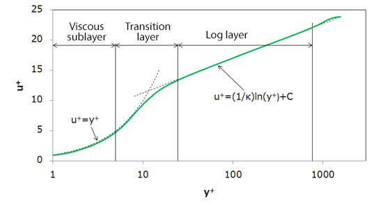
Figure 10.2: Log-law velocity profile

To make use of log-law condition, it is necessary to place the first mesh point from wall in the ‘log layer’, where velocity fits into the log curve. Conversely, if we place the first point in viscous sublayer or in transition layer, thinking that the finer the better, the accuracy of calculation drops because the log-law condition cannot be applied appropriately as wall condition. Generally speaking, there is nothing wrong with finer mesh; however, it is a different story for mesh near wall in a turbulent flow calculation. Care should be taken on the thickness of mesh near wall when you use wall function.

10.3: Turbulence models and wall condition

Log-law is an equation that is created by a combination of theory and experiment, but it holds true only for simple flows such as the one along the walls as shown in the left-hand side of Figure 10.3. If there are bumps on the walls as shown in the right-hand side of Figure 10.3, some portion where log-law does not hold true is created. In such a case, we need to avoid the use of log-law and arrange multiple mesh elements inside viscous sublayer and transition layer. Furthermore, we need to be careful in applying a turbulence model because vortex motions are confined by the walls unlike the regions away from walls, which undermines the premise of normal turbulence models. Turbulence models that are applicable near these walls are called ‘low-Reynolds-number models’. The “low Reynolds number” in this context means the region of slow flows near wall, and it does not mean that this model is used for a flow field having low Reynolds number. Leading examples of low-Reynolds-number models are ‘Abe-Kondo-Nagano (AKN) model’ and ‘Shear Stress Transport (SST) k-ω model’. Note that low-Reynolds-number models are equivalent to normal turbulence models when applied away from walls. That means there is no need to arrange thin mesh for all the walls; instead, you can keep the accuracy near wall by generating thinner mesh only for the regions where log-law is not met or for the regions of interest in terms of near-wall phenomena.

The next column will continue on RANS.

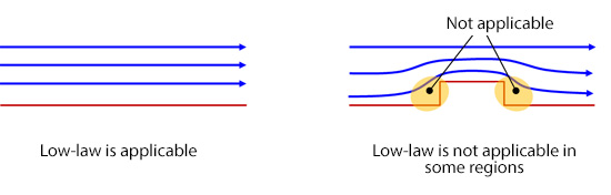
Figure 10.3: Relationship between log-law and flow

About the Author
Takao Itami | Born in July 1973, Kanagawa, Japan

The author had conducted researches on numerical analyses of turbulence in college. After working as a design engineer for a railway rolling stock manufacturer, he took the doctor of engineering degree from Tokyo Institute of Technology (Graduate School of Science and Engineering) through researching compressible turbulent flow and Large-Eddy Simulation. He works as a consulting engineer at Software Cradle solving various customer problems with his extensive experience.