
Basic Course on Turbulence and Turbulent Flow Modeling 9: 9.1 Example of RANS calculation, 9.2 Comparison of turbulence models
Methods of turbulent flow calculation (3)
Example of RANS (Reynolds-Averaged Navier-Stokes) calculation
9.1: Example of RANS calculation
In the previous column, we covered the overview of RANS. In this column, we discuss an example of RANS calculation. We take a flow analysis of engine valves shown in Figure 9.1 as the example. Engine valves are located at the exit/entrance above a piston, and they are crucial components that control the timing of intake and exhaust. With a flow analysis around the valves, we can predict air resistance (pressure loss) across the valves as well as the fluid mixing performance.
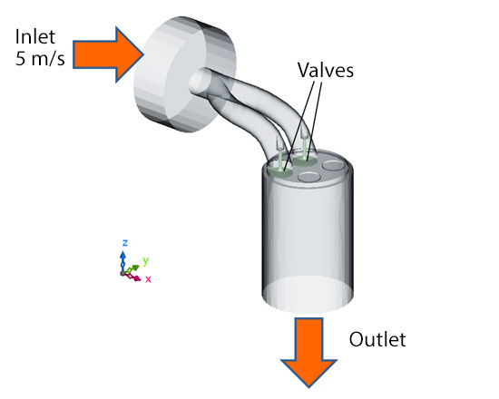
Figure 9.1: Flow analysis model of engine valves
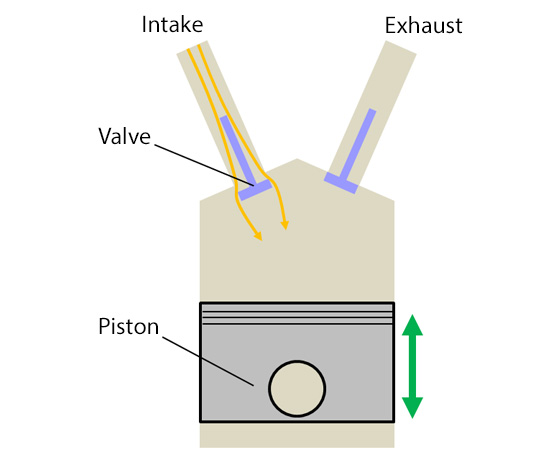
Figure 9.2: Engine valves
Figure 9.3 shows generation of eddies near the valves analyzed by LES (Large-Eddy Simulation). The subsequent columns will explain LES in details; in the simple terms, LES is a calculation method that directly calculates vortex tubes of the sizes greater than mesh size and takes account for the influence of smaller vortex tubes with modeling. The figure illustrates generation of many small vortex tubes as the flow passes through the valves and becomes turbulent. I (and only I?) find the result like Figure 9.3 interesting because it “looks just like the real phenomenon”, but the calculation takes long even with a parallel-computing machine. When design engineers are conducting many case studies, they prefer methods with shorter calculation time and hence RANS is more utilized. Figure 9.4 shows the result of flow analysis with RANS (standard k-ε model). Since a time-averaged field is calculated in RANS, a time-averaged result of LES is shown for comparison. You can see that the flow fields are quite similar. Unfortunately, motions of vortex tubes cannot be captured with RANS, yet it is enough for the purpose of knowing the pressure difference across the valves or the overall flow characteristics. Calculation time of RANS is between one tenth and a few tenth of LES; therefore, RANS is a calculation method suited for performing many case studies with different conditions and/or different valve geometries.
Figure 9.3: Vortex tubes near the valves analyzed by LES
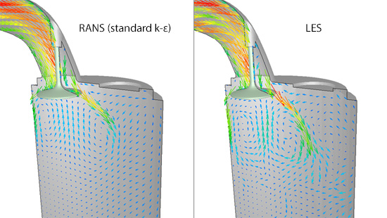
Figure 9.4: Comparison of flow near the valves
Next, let us look at the distribution of eddy viscosity obtained with the RANS calculation. As you can see in Figure 9.5, there is a region of large eddy viscosity downstream of the valve, which coincides with the region where many vortex tubes are generated in the LES calculation. In actuality, the flow field is turbulent with generation of many vortex tubes as in the result of the LES calculation. As a result of considering their effect with eddy viscosity in the RANS calculation, we can say that the average velocity field obtained is comparable to LES.
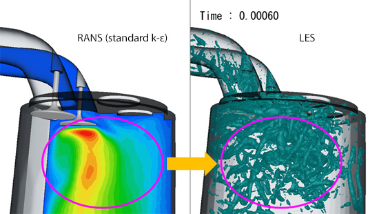
Figure 9.5: Distribution of eddy viscosity (left) and vortex tubes (right)
9.2: Comparison of turbulence models
In RANS model, eddy viscosity is calculated by a ‘turbulence model’. Let us see how the calculation results change with different turbulence models. Figure 9.6 shows a comparison of flow vectors for standard k-ε model and the same model with Kato-Launder correction. There is hardly any difference between them. The next figure is a comparison of turbulence energy distribution (Figure 9.7). For standard k-ε model, there is a local maximum of turbulence energy where the flow impinges on the valve from below. On the contrary, there is no such distribution for the model with Kato-Launder correction. This is the result where standard k-ε model estimates “generation of turbulence” because velocity changes abruptly when the flow hits the wall and velocity difference becomes large.
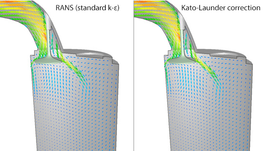
Figure 9.6: Comparison of flow velocity vectors
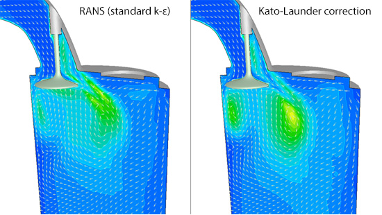
Figure 9.7: Comparison of turbulence energy
Figure 9.8 shows an animation of vortex tube distribution with LES, viewed from below the valves. You can see the white space directly below the valves, which indicates vortex tubes are not generated. In sum, although the different turbulence models did not affect the flow fields in this calculation, they did affect the predicted results of turbulence energy, and the model with Kato-Launder correction made a decent prediction similar to LES. The reason why the turbulence energy distribution did not affect the flow field may be that the flow stagnated below the valves.
In the next column, we will discuss wall conditions of RANS model.
Figure 9.8: Vortex tubes below the valves (LES)

About the Author
Takao Itami | Born in July 1973, Kanagawa, Japan
The author had conducted researches on numerical analyses of turbulence in college. After working as a design engineer for a railway rolling stock manufacturer, he took the doctor of engineering degree from Tokyo Institute of Technology (Graduate School of Science and Engineering) through researching compressible turbulent flow and Large-Eddy Simulation. He works as a consulting engineer at Software Cradle solving various customer problems with his extensive experience.

