Methods of turbulent flow calculation (5)
Sample calculations using low-Reynolds-number model

11.1: Back-step flow

In the previous column, we covered log-law, one of the wall conditions of RANS model. We learned that log-law is a technique for making near wall mesh coarse by placing the first mesh point within the ‘log layer’ and by applying the log-law condition as wall condition. We also learned that we would use low-Reynolds-number model to accurately calculate the regions where log-law does not hold true, e.g., bumpiness on the walls, by arranging mesh very close to the walls (inside viscous sublayer and transition layer) with higher resolution near wall. This time, let us discuss the effectiveness of low-Reynolds-number model with specific sample calculations. The first example is a flow field called ‘back-step flow’. As shown in Figure 11.1, the flow field is such that the flow comes in from the left and goes over a step downstream. The analysis condition is given by Reynolds number of 46,000 based on the inflow velocity U and step height H. The flow is along the walls until the step, then it draws apart from the walls --- so-called separation --- and it again flows along the walls after some distance, which is called a reattachment phenomenon. This analysis focuses on the distance from the step to the location of reattachment, or the reattachment distance. Presumably, the log-law condition does not hold true in the region behind the step, where the flow is not along the walls.

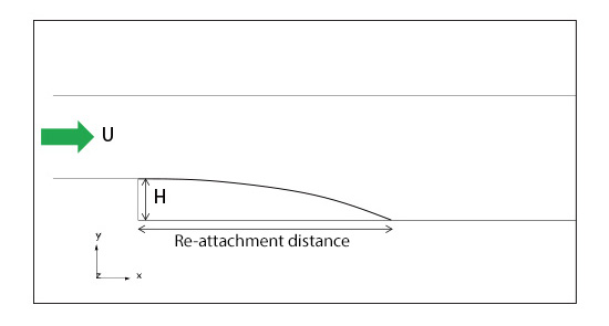
Figure 11.1: Back-step flow

Figure 11.2 shows the calculation results with standard k-ε model and two low-Reynolds-number models: AKN model and SST k-ω model. The ‘streamlines’ are displayed to visualize the flow patterns. While there are differences in the distances to the reattachment points, all the turbulence models gave the results in which the flow separates at the step and reattaches downstream. These results indicate that, because the presence of the step determines the separation point in this case, no qualitative discrepancy is produced by different turbulence models even if the log-law does not hold true behind the step.

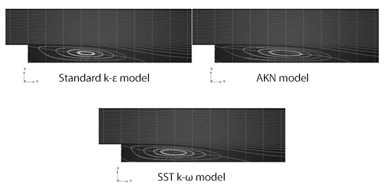
Figure 11.2: Comparison of back-step flow by turbulence models

11.2: Flow around airfoil

The second example is a flow around a cross-section of airplane wing, or ‘flow around airfoil’. This is a calculation to predict lift force generated by the wing or to investigate a possible stall. This particular example assumes a situation where the angle between the wing and wind direction is 14 degrees, as shown in Figure 11.3. Since airplane wings are made with smooth, gradual curves, it is difficult to predict in advance where the separation occurs, unlike the back-step flow in 11.1. Under this condition, we can expect some qualitative differences in the flow depending on turbulence models.

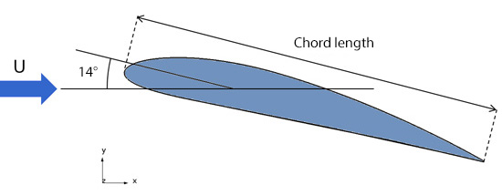
Figure 11.3: Analysis of flow around airfoil

Figure 11.4 shows the streamlines for the calculation results with the three turbulence models. There is an angle between the wing and the flow direction in this example, and it was confirmed by actual measurement that the separation did occur on the rear top surface of the wing. In the result with SST k-ω model, we can see the separation; on the other hand, there is no separation with standard k-ε model or AKN model. Despite being categorized as the same low-Reynolds-number model, AKN model cannot predict the separation that occurred in the actual phenomenon. This indicates that, in order to simulate a separation, simply refining mesh near wall cannot replicate the phenomenon unless the turbulence model is appropriate. While AKN model is an extension of standard k-ε model, SST k-ω model employs the k-ω model near wall, which is better at predicting separations. This may be why the latter model was able to predict the separation on the wing surface when the former model could not.

As illustrated in this example, SST k-ω model is a good model for predicting ‘separation’. In other cases, however, it may or may not be as accurate. The reality is there is no single turbulence model that is highly accurate in every application. While on the other hand, there is a calculation method which tries to overcome this issue by not relying on turbulence models when flows can be captured with mesh: LES (Large Eddy Simulation). We will cover LES in the next column.

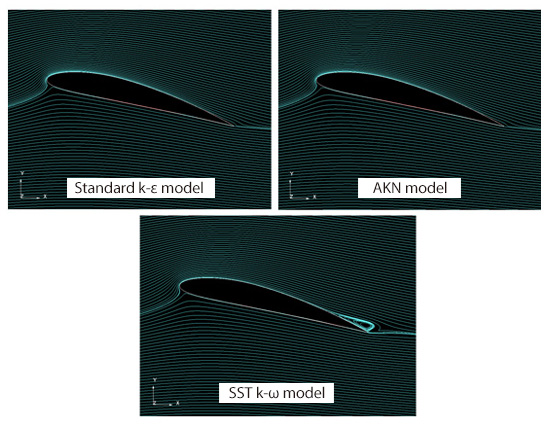
Figure 11.4: Comparison of flow around airfoil by turbulence models

About the Author
Takao Itami | Born in July 1973, Kanagawa, Japan

The author had conducted researches on numerical analyses of turbulence in college. After working as a design engineer for a railway rolling stock manufacturer, he took the doctor of engineering degree from Tokyo Institute of Technology (Graduate School of Science and Engineering) through researching compressible turbulent flow and Large-Eddy Simulation. He works as a consulting engineer at Software Cradle solving various customer problems with his extensive experience.