Solidification/melting analysis I

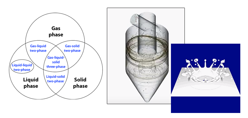
Solidification/melting analysis is an example of liquid-solid two-phase flow analyses. For a micro approach of solidification phenomena, modeling of processes of solidification core generation and crystal growth is required, however, unfortunately there is no general-purpose analysis method. Therefore, consider a macro approach instead.

The volume fraction of solid phase in the fluid is defined as the solid phase rate. It is assumed to be balanced on the solid-fluid interface, and the change of the solid phase rate is obtained with the temperature recovering method. As shown in Figure 1, the temperature of the fluid element is solved. If the temperature is lower than the liquidus temperature (same as the solidus temperature with a pure substance like water if it is balanced), the solid phase rate is calculated from the latent heat and the specific heat. Then, the temperature of the fluid element is recovered by releasing the latent heat (generating heat) corresponding to the solid phase rate and solving the temperature of the fluid element again. The solid phase rate and temperature of the fluid element can be obtained by repeating this.

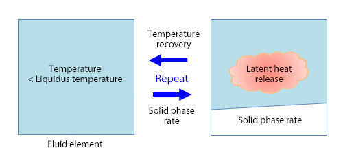
Figure 1: Temperature recovering method

Here is an analysis example. Natural ice made in a water pond in winter is analyzed. It is said that natural ice grows from the water surface of a water pond when cold air remains for about 20 days and the thickness that can be cut becomes 15 cm or more. To see if it can be reproduced, solidification/melting analysis is conducted.

As shown in Figure 2, a water pond with length of 24 m, width of 14 m, and depth of 0.5 m is considered. The pond is surrounded by curb stones and organic soil. The ambient temperature of the upper surface of the pond is -8^° C, and the coefficient of heat transfer is 10 W/(m² K). The temperature of the under surface of the pond is 4^° C, which is a heat conduction condition. Under this condition, unsteady analysis for 20 days is conducted. The flow of water is not solved.

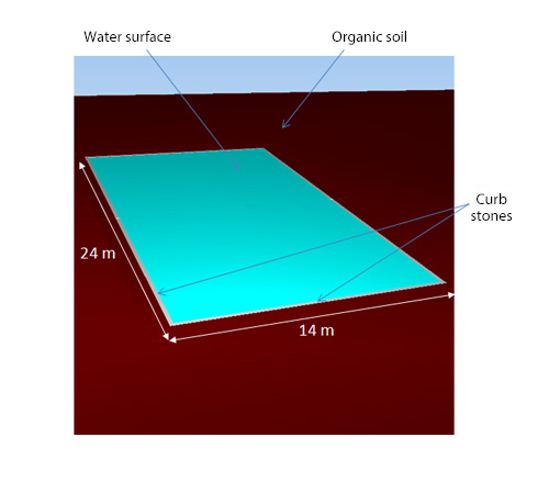
Figure 2: Water pond

Figure 3 shows the temporal change of water surface temperature distribution until two hours later. The temperature lowers on the water surface almost evenly. When about one hour and a half have passed, the water surface temperature becomes 0^° C and fixed. Figure 4 shows the temporal change of solid phase rate distribution in the depth section of the central part of the water pond. It shows that ice grows from the water surface. The red dotted line in Figure 4 shows a position 15 cm beneath the water surface. You can see that the thickness of the ice has reached 15 cm after 20 days (480 hours).

Figure 3: Temporal change of water surface temperature distribution (fresh water)

Figure 4 Temporal change of solid phase rate distribution in section of central part of water pond (fresh water)

Then, what happens if the water in the water pond is salt water like seawater instead of fresh water? Seawater is mixture with salinity concentration of 3.4% (mass fraction), and the water starts freezing at ‐1.8^° C (liquidus temperature). The salt content starts freezing at ‐21^° C （solidus temperature), which is called eutectic point. Unsteady analysis is conducted again in consideration of this.

Figure 5 shows the temporal change of water surface temperature distribution until two hours later. Figure 6 shows the temporal change of solid phase rate distribution in the depth section of the central part of the water pond. As shown in Figure 6, the ice stops growing, and decrease of solidifying point with salt content is reproduced. In Figure 7, the solid phase distribution in the section of the central part of the water pond is displayed by changing the upper limit to 0.25. It shows that the solid phase rate is 0.25 near the water surface and 0.10 at the depth of 15 cm even in the case of salt water. You can imagine a state in which ice blocks are floating here and there in salt water.

Figure 5: Temporal change of water level temperature distribution (salt water)

Figure 6: Temporal change of solid phase rate distribution in section of central part of water pond (salt water)

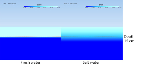
Figure 7:　Solid phase rate distribution in section of central part of water pond 20 days later

The times in animations in Figures 3 and 5 are accelerated by 600 times, and the times in animations in Figures 4 and 6 by 288,000 times. The next section will explain solidification/melting analysis in which the flow is analyzed simultaneously.

---

About the Author 
Katsutaka Okamori | Born in October 1966, Tokyo, Japan

He attained a master’s degree in Applied Chemistry from Keio University. As a certified Grade 1 engineer (JSME certification) specializing in multi-phase flow evaluation, Okamori contributed to CFD program development while at Nippon Sanso (currently TAIYO NIPPON SANSO CORPORATION). He also has experience providing technical sales support for commercial software, and technical CFD support for product design and development groups at major manufacturing firms. Okamori now works as a sales engineer at Software Cradle.