
Master Course for Fluid Simulation Analysis of Multi-phase Flows by Oka-san: 8. Particle tracking analysis II
Particle tracking analysis II
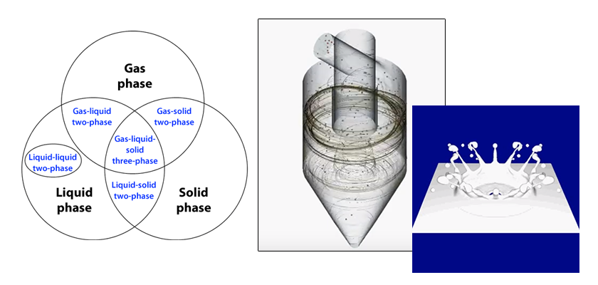
This section describes condition settings for the particle tracking method. The particle tracking method is one method used for particle simulation analyses.
An accurate multi-phase analysis for sand or dust particles, where particle diameters are often less than 1 mm, requires using a large number of particles in the simulation. However, the number of particles which can be analyzed in a multi-phase flow analysis is limited by the time available to complete the calculations and the computer hardware capabilities. To compare the impact of the particle diameter to the number of particles needed to attain accurate results, the following example is used. For a particle density of 2,500 kg/m3 and particle diameters of 100 μm, 1 g of the particles consists of 760,000 particles. For 1 g of the particles with diameter of 10 μm, the number of particles in 1 g is 760 million. Analyzing such large number of particles is not realistic for a two-way coupled analysis (analysis where the fluid and particles affect each other). However, if a one-way coupled analysis (where the fluid affects the particles but the particles do not affect the fluid) described in the previous section can be used, an enormous number of particles can be analyzed reasonably and efficiently. The one-way coupled analysis can be useful for qualitative analyses.
In a two-way coupled analysis, which is a quantitative analysis, an effective number of particles must be specified. This number equates to a specific number of particles obtained based on a certain mass of a representative particle that will be tracked. This is called the Parcel approximation.
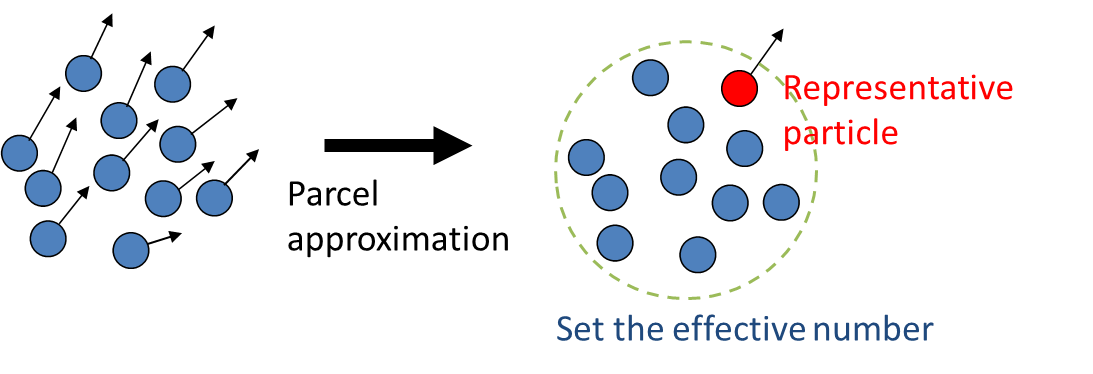
Figure 1: Parcel approximation
The condition settings used to define when particles reach a boundary face depend on how the software is programmed. Typical boundary face conditions are shown in Figure 2. The most frequently used condition is repulsion. After particles reach a boundary face, their behavior changes depending on the repulsion coefficient. The “adhesion” condition is effective when evaporation or volatilization of particles is considered at a boundary face. The “vanishment” condition removes particles that reach a boundary face. “Vanished” particles are no longer tracked in the calculations and reduce the calculation load (although the number of vanished particles can be separately counted). The “moves along with a wall” condition is applied to particles which are not “repulsed” but move along a boundary wall.
Figure 2: Boundary face conditions
Top left: repulsion coefficient of 1.0, top right: repulsion coefficient of 0.5
Bottom left: adhesion or vanishment condition, bottom right: moving along with a wall
Another condition setting is needed to simulate the effects of turbulence fluctuations on the particles. The Reynolds Averaged Navier-Stokes (RANS) turbulence model cannot express turbulent flow variations of particles. Figure 3 shows an analysis result for particles rising due to buoyancy. A RANS turbulence model is used in the flow analysis and the particle tracks are the same for all particles with the same starting position and initial condition. Turbulence should cause the particles to take different paths. To express the turbulent flow variation of the particles, a turbulent flow variation obtained from the turbulence model is added to the velocity of the particles by using random numbers. By using this method, the calculated particle tracks will be different for each particle even though the particles starting positions and initial condition are the same.
Figure 3: Turbulent flow variation
left: without turbulent flow variation, right: with turbulent flow variation
Consider an example to demonstrate condition settings for a particle tracking analysis. Trees are used to form a snowbreak to provide improved visibility for vehicles on the road during a snowstorm. As shown in Figure 4, the trees used for the snowbreak are narrow-band woods and consist of evergreen trees. Air at -20°C flows into the computational domain at a speed of 8 m/s with the reference height of 10 m using a power-law profile (appropriate for flat land). In addition, snow particles with a density of 200 kg/m3 and diameter of 100 μm flow into the computational domain uniformly up to a height of 3 m from the ground. Parcel approximation is applied to the analysis (two-way coupled). The effective number of snow particles is 1,000. The repulsion coefficient against boundary faces such as the ground and windbreak fences is 0.5. To count the snow particles, three regions are set: the snowstorm region (from the inlet to the windbreak fences), the snowbreak region (from the fences to the embankment), and the road region (the residual region). The analysis is performed for an 8 second period.
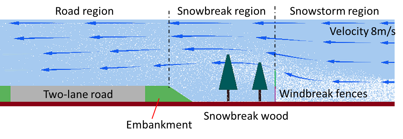
Figure 4: Snowbreak woods on road
As shown in Figure 5, the evergreen trees are geometrically represented with conical bases. They are set as a pressure loss region with a leaf area density of 8 m2/m3 and a resistance coefficient of 0.7. The repulsion coefficient of the snow particles on the needle-leaf surface of the trees is 0.1. The evergreen trees are arranged in a zigzag pattern with a spacing of 4 m (narrow-band region). Creating forests like these takes a long time. As shown in Figure 6, three periods are set in this analysis: nursery period (15 years after planting), rearing period (15 years after nursery period), and conservation period (more than 30 years after planting). During the nursery period, additional snowbreak fences are set on top of the windbreak fences. The windbreak fences do not have any openings. The opening ratio of the snowbreak fences is 30%.
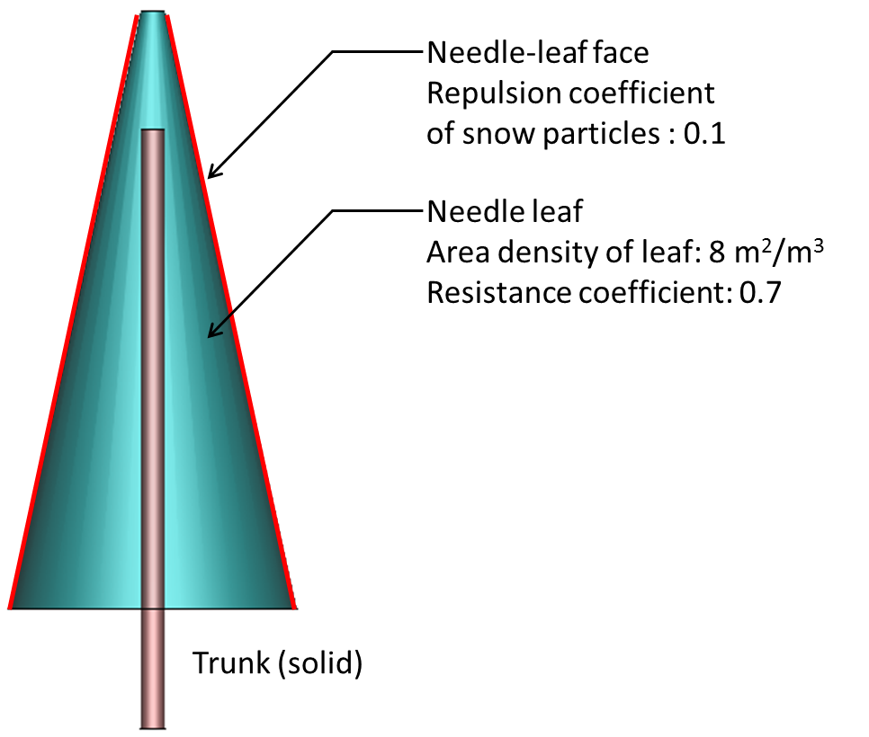
Figure 5: Needle-leaf tree (Cross section)
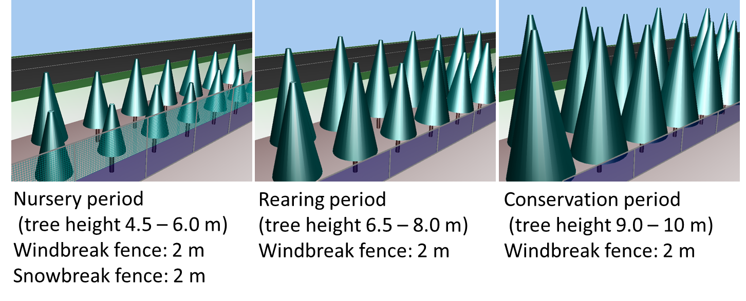
Figure 6: Narrow-band woods
Figure 7 shows the analysis results for the snow particles in each period. The difference between the periods is accurately simulated.
Figure 7: Snow particles in nursery period (Top), Snow particles in rearing period (Middle),
Snow particles in conservation period (Bottom)
Figure 8 shows the time variation of the number of snow particles. The number of snow particles is counted in the snowstorm region, snowbreak region, and road region. As the snowbreak woods grow, the number of snow particles in the snowbreak region increases and the number of particles in the road region decreases. This shows that the snowbreak effectiveness increases with years.
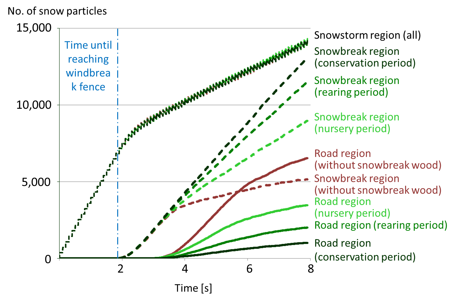
Figure 8: Time variation of the number of snow particles
Figure 9 shows the visibility on the road with and without the snowbreak forests (conservation period). The snowbreak forests clearly improve visibility on the road.
 |
 |
In the next section, evaporation and volatilization of particles will be discussed.

About the Author
Katsutaka Okamori | Born in October 1966, Tokyo, Japan
He attained a master’s degree in Applied Chemistry from Keio University. As a certified Grade 1 engineer (JSME certification) specializing in multi-phase flow evaluation, Okamori contributed to CFD program development while at Nippon Sanso (currently TAIYO NIPPON SANSO CORPORATION). He also has experience providing technical sales support for commercial software, and technical CFD support for product design and development groups at major manufacturing firms. Okamori now works as a sales engineer at Software Cradle.

