Free surface flow analysis IV

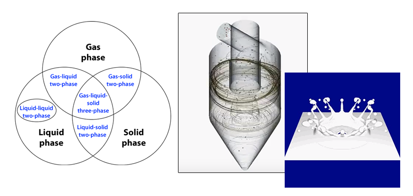
　This chapter discusses calculation time, which is an important consideration when free surface problems are solved using the VOF method.

　Since free surface flow analyses using the VOF method are transient analyses, they require more calculation time than steady-state analyses. If the calculation is unstable, the time step (or Courant number) must be reduced. To prevent interface diffusion caused by numerical calculation error, the mesh near the interface must have fine resolution. The calculation time will increase for both of these cases.

　Different methods can be used to reduce the calculation time. One of the methods will be introduced by showing an analysis example.

In this example, oil sloshing in an oil tank due to an earthquake will be analyzed. As shown in Figure 1, the oil tank is 42.7 m in diameter and 24.4 m high. Its maximum capacity is 30,000 kL of oil. In this example, 26,000 kL of oil (density: 740 kg/m³ , viscosity: 0.0026 Pa∙s, surface tension coefficient: 0.020 N/m) is stored. The oil level height is 18.2 m. The tank shakes laterally with a lateral acceleration of 1 m/s² for 10 seconds. The movement is caused by a long-period earthquake ground motion with a period of 5 seconds. A structural mesh with 1,306,800 uniform elements is used for the inside of the tank, and the analysis is performed using the MARS (Multi-interface Advection and Reconstruction Solver) method for 60 seconds in real time. The time step is automatically set so the Courant number will not exceed 0.9.

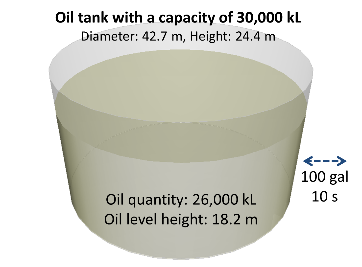
Figure 1: Oil tank with a capacity of 30,000 kL

Figure 2 shows the analysis result, for the behavior of the oil surface. When the background is blue, the tank is shaking for 10 seconds. When the background is white, the tank remains stationary for 50 seconds. Figure 2 shows that the oil surface reaches the highest position several seconds after the earthquake stops. The oil surface gradually lowers; however, sloshing continues even after 60 seconds. The analysis calculation time to produce these results is approximately 4 hours. Actual time will depend on the program code and the computers used.

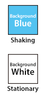Figure 2: Analysis result – Behavior of the oil surface

 

　What can be done to reduce the calculation time? Since the earthquake motion is laterally unidirectional, a symmetry plane can be defined as shown in Figure 3. When the symmetry plane is used, the number of elements can be reduced in half and the calculation time by over 50%.

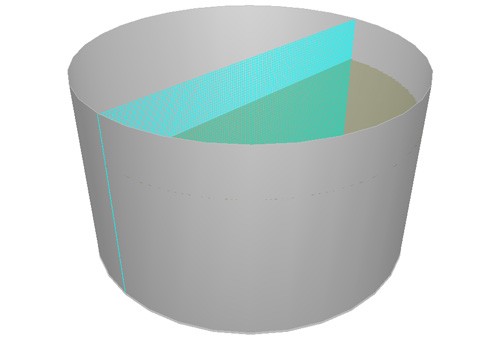
Figure 3: Symmetry plane

　Another way to reduce the calculation time is to take advantage of parallel processing. In this example, the program code can be parallelized by MPI (Message-Passing Interface) or another method in combination with the hardware computing platform using a multi-core CPU. Parallel computing has the potential to reduce the current calculation time by 47%.

　To further reduce calculation time, a coarser mesh can be used without decreasing the calculation accuracy. As shown in Figure 4, a coarser mesh can be used outside of the maximum distance the interface moves. This can reduce the number of elements down to 505,296 which will decrease calculation time by over 20%

 

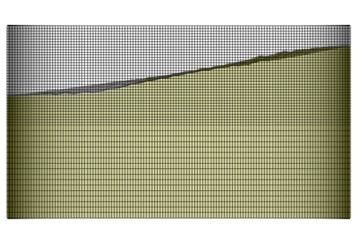
Figure 4: Element distribution

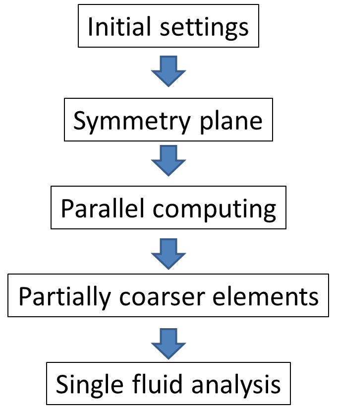
Figure 5: Operation flow for reducing the calculation time

　Some program codes are capable of analyzing this phenomenon as a single fluid analysis. As long as the liquid does not engulf the gas in a sloshing analysis, the analysis can be treated as a single phase analysis. If this is possible, the calculation time can be reduced by 30%.

　Figure 5 shows the operation flow for reducing the calculation time. The calculation time is 86% shorter than that required in the initial settings if all the methods explained above are implemented. In practical terms, the analysis that initially took 4 hours to run could now be completed in 30 minutes. To check the calculation accuracy between the two approaches, the analysis results (the behavior of the oil surface) are compared as shown in Figure 6. The figure on the left shows the behavior of the oil surface after the calculation time is reduced and on the right before the calculation time is reduced. The red line indicates a height 3.5 m above the initial oil level. The figure shows that the behaviors of both surfaces are almost identical.

Figure 6: Comparison of the analysis results
(Left: After reducing the calculation time, Right: Before reducing the calculation time)

　For the next calculation, the period of the lateral shake is changed from 5 seconds to 4 seconds and 2 seconds. The duration of the shaking is unchanged: 10 seconds. Figure 7 shows the behavior of the surface when the period of lateral shake changes. The period for the figure on the left is 2 seconds, and the period on the right is 4 seconds. Both oil level heights do not exceed the red line set at 3.5 m. This indicates that both oil levels are lower when the period of lateral shake is reduced. In addition, both figures show that sloshing is attenuated and the surface stops shaking after 60 seconds. Considering the period of 5 seconds, resonance occurs because the 5 second period is close to the natural period of sloshing.

Figure 7: Comparison of the analysis results with different periods (Left: 2 seconds, Right: 4 seconds)

　The next column will be the last one as for free surface flow analyses. I will introduce an analysis example of a micro scale free surface flow.

---

About the Author 
Katsutaka Okamori | Born in October 1966, Tokyo, Japan

He attained a master’s degree in Applied Chemistry from Keio University. As a certified Grade 1 engineer (JSME certification) specializing in multi-phase flow evaluation, Okamori contributed to CFD program development while at Nippon Sanso (currently TAIYO NIPPON SANSO CORPORATION). He also has experience providing technical sales support for commercial software, and technical CFD support for product design and development groups at major manufacturing firms. Okamori now works as a sales engineer at Software Cradle.