Free surface flow analysis III

This chapter continues the discussion about the VOF method and contains additional analysis examples.

In the VOF method, the volume fraction of a fluid occupying each element of the computational domain is defined by the F value, and the transport equation is solved using the F values. During the calculation, an extremely small F value can appear as shown in Figure 1. To avoid the cancellation of significant digits, double precision should be used. Moreover, a cut off value for F must be defined for a stable calculation. How the cut-off value for F value is processed will depend on the program code. If a cut off value is not used, the volume of the liquid will decrease over time, even though the computational domain is closed.

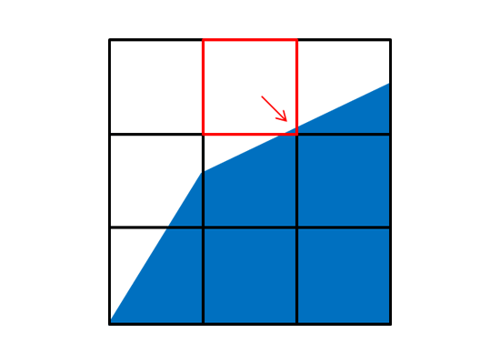
Figure 1: Cut-off F value

Another important consideration about VOF is calculation stability. In a transient analysis, when the fluid flows beyond the element width L within the time step t, the calculation becomes unstable. When the calculation is unstable, the interface will fluctuates significantly. The solution is to reduce t to a smaller value. This can also be achieved by setting Courant number C to a value less than 1 when t is automatically set by C as shown in Figure 2.

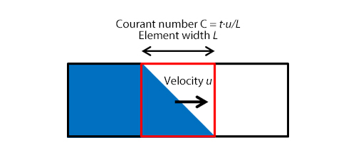
Figure 2: Courant number

In the latest fluid simulation analysis software, a combination of VOF and other analysis functions are used to analyze free surfaces. This enables a free surface flow with phase change or with moving objects to be analyzed. An analysis example of a free surface flow with a moving object (rigid body) will be discussed.

Two methods for a flow simulation analysis with a moving object are considered:

• Overset mesh method that overlaps the moving region elements and the stationary region elements (Figure 3)
• Element deformation and regeneration method that eliminates the need to separate the moving region and the stationary region

The overset mesh method has a significant advantage: the program will be simpler and the calculation will be stable because the elements do not need to be regenerated. To increase the calculation accuracy, the element distribution (refinement level) must be equal at in overlapping region between the moving and stationary regions.

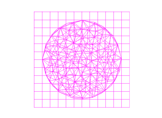
Figure 3: Overset grid

An amusement park water ride is a free surface/rigid body example that can be analyzed using the overset mesh method. Water ride attractions are always popular rides at amusement parks. They are popular because of the thrill created by the seemingly unpredictable up and down motion of the ride vehicle and surprising splashes which cause the passengers to get wet. The velocity and the inclination of the ride vehicle are highly affected by its weight and center of gravity, and also the water stream. A fluid simulation analysis can be very useful for predicting the vehicle’s motion.

The motion of the amusement park ride vehicle is analyzed using the combination of VOF and overset mesh. In the analysis, the 6DOF (6 degrees of freedom) momentum equation is solved. By solving the equation, the vehicle translates and rotates depending on the force from the water stream that acts on the vehicle.

Figure 4 shows the attraction model. The total length of the watercourse is 15 m, and the widths of the entrance and exit are 5.5 m and 6.5 m, respectively. The water depth is 1.5 m. The ride vehicle has a diameter of 3 m and can accommodate up to 4 adults (Figure 5). The weight of four passengers is considered by assigning each seat a weight of 86 kg. For security, a handrail is placed at the center of the vehicle and the vehicle is enclosed with a safety fence. To enable the vehicle to float on the water, the density of the lower column and the surrounding safety fence is set to 360 kg/m³ . The velocity of the ride vehicle will be controlled by the water stream.

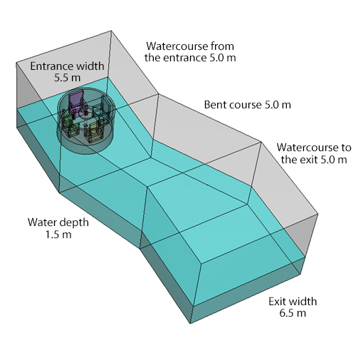
Figure 4: Bent watercourse

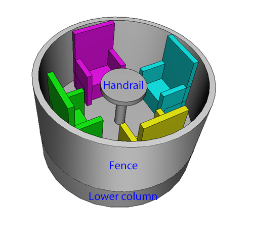
Figure 5: Ride vehicle with a diameter of 3 m

Figure 6 shows the analysis result of the ride vehicle traveling on the water at 6 km/h. The ride vehicle pitches and rolls as shown in Figure 6. Figure 7 shows the analysis result at 7 km/h. The vehicle does not capsize; however, it careens freely and the risk for the passengers increases.

Figure 8 shows the relation between the height of the vehicle on the water and the distance traveled. The height difference is 0.54 m after the vehicle travels 10 m at 6 km/h, and it reaches 1.2 m at 7 km/h. At 6 km/h, the vehicle strongly pitches and rolls, and 6 km/h is sufficient speed to make the water ride fun and exciting.

Figure 6: Ride vehicle traveling on the water (Velocity: 6 km/h)

Figure 7: Ride vehicle traveling on the water (Velocity: 7 km/h)

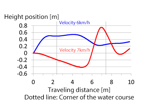
Figure 8: Relation between the height position of the vehicle and the traveling distance

The next column will explain the calculation time, which is an important issue of VOF method.

---

About the Author 
Katsutaka Okamori | Born in October 1966, Tokyo, Japan

He attained a master’s degree in Applied Chemistry from Keio University. As a certified Grade 1 engineer (JSME certification) specializing in multi-phase flow evaluation, Okamori contributed to CFD program development while at Nippon Sanso (currently TAIYO NIPPON SANSO CORPORATION). He also has experience providing technical sales support for commercial software, and technical CFD support for product design and development groups at major manufacturing firms. Okamori now works as a sales engineer at Software Cradle.