VOF (volume of fluid) method

　This section describes VOF method, which is a commonly used free surface flow analysis method.

　In the VOF method, a volume fraction of a fluid occupying each element in the computational domain is defined by F where (0 ≤ F ≤ 1). The transport equation is solved to determine the interface. Figure 1 shows an example of the distribution of F values. When F = 0, the material property (e.g., density and viscosity) of the first fluid (e.g., air) predominates. When F = 1, the material property of the second fluid (e.g., water) predominates. When F is between 0 and 1, the material properties of two fluids are weight-averaged by the F value. Therefore, the element near an interface must be small enough to avoid large error.

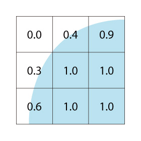
Figure1: Example of distribution of F values

　In SOLA-VOF, a code developed by Los Alamos National Laboratory (US) in the 1970’s, the donor-acceptor method was used for the advection of F values between elements. This method strictly maintained F values; however, this resulted in the interface being expressed in a staircase pattern as shown in Figure 2. Currently, many VOF methods use interface gradients to create a continuous interface. These include the MARS method (Multi-interface Advection and Reconstruction Solver), a new VOF method proposed by Professor Kunugi at the Kyoto University Graduate School.

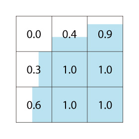
Figure 2: Interface expressed in staircase pattern

　In a free surface flow analysis, the surface tension of a fluid material is important. The VOF method often uses a CSF (Continuum Surface Force) model, where the surface tension acting on an interface is considered a volume force. Consider the effect of surface tension for an “Oil droplet rising in water” introduced in master course No.1 as an example of a liquid-liquid two-phase flow. Figure 3 is an analysis example considering surface tension of the water and oil. Figure 4 is an analysis example in which the surface tension of water and oil is reduced to 1/1000. As shown in Figure 4, when the surface tension is reduced, the rising oil droplets cannot keep their shape.

 

Figure 3: Rising oil droplets

 

Figure 4: Rising oil droplets (with small surface tension)

　In a free surface analysis near a solid surface, the contact angle is also an important parameter. The contact angle is the angle between a wall and a free surface of the fluid as shown in Figure 5. When the contact angle is small, the wall is more hydrophilic. In contrast, when the angle is large, the wall tends to repel the liquid.

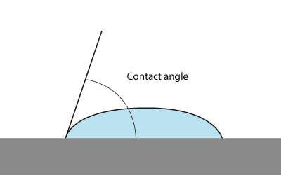
Figure 5: Contact angle

　The effect of the contact angle can be better understood by analyzing capillary action (See Figure 6). Two plates, whose walls are hydrophilic with a contact angle of 60 degrees, are separated a distance of 1 mm from each other (Left figure). The figure on the right shows two plates whose walls are water-repelling with a contact angle of 120 degrees. Both sets of plates are immersed into water. For simplification, the contact angles are only defined for the facing surfaces of the plates. As shown in Figure 6, due to capillary action, the water level rises between the plates with hydrophilic walls and falls between the plates with the water repelling walls. The fluid behavior largely depends on the contact angles.

Figure 6: Capillary

　Another analysis example can further illustrate capillary action. A percolation phenomenon in soil is analyzed using the MARS method. As shown in Figure 7, the cross-section of the soil (depth: 30 mm, width: 70 mm) is considered. The soil level dips 1 mm in the center. The soil is made up of sand, with porosity of 0.15, and a Darcy’s coefficient of 5 x 10^-10 m² . A water level of 0.5 mm (uniform height) is set as the initial condition. The height at the center is 1.5 mm. Then, percolation phenomenon is simulated.

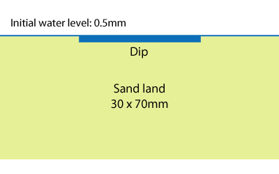
Figure 7: Analysis target

　Figure 8 shows the analysis result after 2 seconds. The superficial velocity at the center is approximately 10 mm/s. Figure 9 shows another analysis result. Here, resin is used (contact angle: 90 degrees, porosity: 0.15) with a Darcy’s coefficient 100 times smaller than that of sand, which increases the water retention ability of the soil. The resin is at the depth of 5 mm. The result shows that percolation is prevented by the resin (shown in green). Resin applications such as this are studied to promote greening of deserts and to prevent desertification.

Figure 8: Percolation into land

Figure 9: Percolation into land (with resin)

---

About the Author 
Katsutaka Okamori | Born in October 1966, Tokyo, Japan

He attained a master’s degree in Applied Chemistry from Keio University. As a certified Grade 1 engineer (JSME certification) specializing in multi-phase flow evaluation, Okamori contributed to CFD program development while at Nippon Sanso (currently TAIYO NIPPON SANSO CORPORATION). He also has experience providing technical sales support for commercial software, and technical CFD support for product design and development groups at major manufacturing firms. Okamori now works as a sales engineer at Software Cradle.