Free surface flow analysis

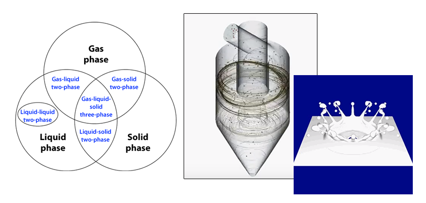
　Among the many types of multi-phase flow simulations, the free surface flow simulation is one of the most frequently modeled simulations. It can be adapted to many target models such as gas-liquid two-phase flows, liquid-liquid two-phase flows, and gas-liquid-solid three-phase flows. Furthermore, the interface behavior obtained from the simulation can be tested using visualization experiments.

　There are two methods to analyze a free surface flow: interface capturing method and interface tracking method. The interface capturing method simulates interface behavior by using advection of a function that represents the interface (Figure 1). Major interface capturing methods are Marker and Cell (MAC), Level Set, and Volume of Fluid (VOF).

　In comparison, the interface tracking method simulates the interface behavior by deforming the elements representing the interface (Figure 2). A commonly used interface tracking method is the Arbitrary Lagrangian and Eulerian (ALE) method. The Particle Method can be regarded as a type of interface capturing method.

Figure 1: Interface capturing method

Figure 2: Interface tracking method

　The interface tracking method more accurately simulates the interface behavior than the interface capturing method does. However, the interface tracking method may require re-generation of the elements based on the interface fluctuation. In addition, the calculation can become unstable as the elements are deformed due to a large degree of fluctuation of the interface. (This problem can be avoided by increasing the number of elements; however, the calculation load will increase.)

　Today many fluid simulation software products are using the VOF method for free surface flow analyses. The reasons are as follows:

　

• SOLA-VOF, developed by Los Alamos National Laboratory, is publicly available and can be integrated into existing fluid simulation software.
• The software coding is relatively simple because elements do not need to be re-generated.
• The calculation is stable even when the interface fluctuates substantially. 　

 

　Consider an analysis example. An air lift pump is used to draw water from wells and hot springs. A free surface flow analysis can be performed for an air lift pump using the Multi-interface Advection and Reconstruction Solver (MARS) method. This is a type of interface capturing method.

　Figure 3 conceptually illustrates an air lift pump. The lower part of a pipe (lifting pipe) is submerged and air is introduced into the pipe. The water in the pipe is mixed with the air and its specific gravity decreases. Then, the water is pumped above the water surface. Air lift pumps are widely used because they are simple and are not easily broken. The pump output is empirically calculated based on the amount of the delivered air, the submergence depth, and the pump head height. Depending on what the pump is used for, aeration can also be provided. To provide aeration into the pump, the flow pattern of the gas-liquid two-phase flow in the lifting pipe must be known (Figure 4). A visualization experiment is the best way to determine the flow pattern; however, practical implementation of such an experiment is extremely difficult. Therefore, fluid simulation is an alternative method for visualizing the flow pattern in the pipe.

 

Figure 4: Flow patterns of a gas-liquid two-phase flow in a pipe

　The pump analysis consists of a rectangular lifting pipe with a width of 5 cm and a rectangular air pipe with a width of 2 cm. The tip of the air pipe has four air inlets in a staggered array. The pump is located 1 m beneath the water surface and draws water into a container located at 10 cm above the water surface. The air flows into the pipe at a rate of 25 L/min every 0.1 second. Figure 6 shows the analysis result. The gas-liquid interface is considered an isosurface. The simulation results show the air/water mixture is drawn up through the lifting pipe and sprayed into the container. Figure 7 shows the distribution of air and water at the center of a cross section of the lifting pipe. The blue area shows where the water is expressed. This figure suggests the flow in the lifting pipe is a slug flow. Do you agree?

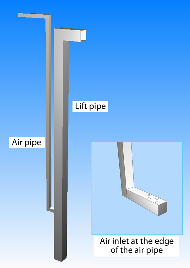
Figure 5: Analyzed pump  

Figure 6: Isosurface

Figure 7: Gas-liquid distribution

　The next column will explain VOF method in detail.

---

About the Author 
Katsutaka Okamori | Born in October 1966, Tokyo, Japan

He attained a master’s degree in Applied Chemistry from Keio University. As a certified Grade 1 engineer (JSME certification) specializing in multi-phase flow evaluation, Okamori contributed to CFD program development while at Nippon Sanso (currently TAIYO NIPPON SANSO CORPORATION). He also has experience providing technical sales support for commercial software, and technical CFD support for product design and development groups at major manufacturing firms. Okamori now works as a sales engineer at Software Cradle.