Methods of turbulent flow calculation (1)
DNS (Direct Numerical Simulation)

7.1: Overview of DNS

This column and the subsequent columns will discuss the methods of turbulent flow calculation. There are mainly three methods of turbulent flow calculation: DNS (Direct Numerical Simulation), RANS (Reynolds-Averaged Navier-Stokes) model, and LES (Large-Eddy Simulation). Let us discuss DNS first.

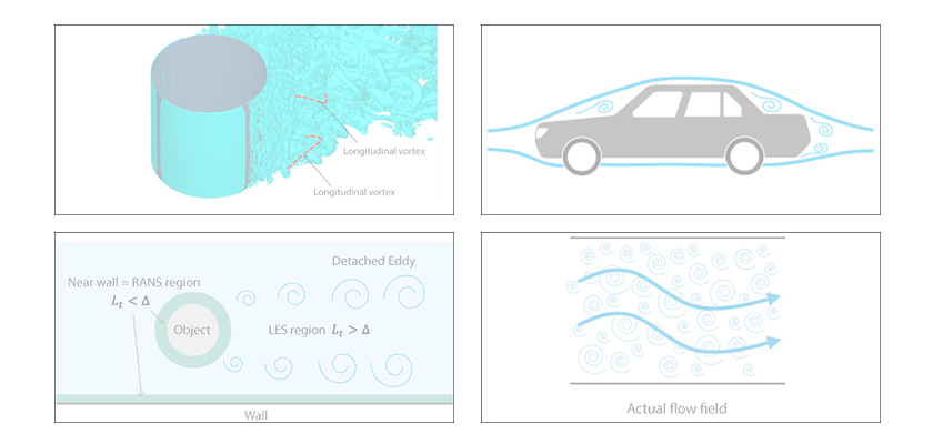
DNS is often referred to as the calculation method without modeling because it “directly solves” the Navier-Stokes equations, the equations of fluid motion. Strictly speaking, however, it does have a modeling because the equations of motion themselves have a model, “viscous force is proportional to the velocity difference”, in them as we learned in Chapter 6. Even so, there is no modeling about turbulence, which is “solved directly”. This requires a calculation with mesh that captures minimum-sized (Kolmogorov scale) eddies, which makes DNS an extensive calculation in general. Moreover, since turbulent flows are essentially transient phenomena, calculations are transient analyses, which take time. It is therefore difficult to use DNS as a practical analysis tool, while DNS is used substantially in researches that examine characteristics of turbulent flows. That is to say, it is cost-consuming to measure eddies in experiments, and conditions that can be tested are limited, whereas numerical simulations have a merit of enabling calculations with a higher degree of freedom in terms of conditions as well as allowing all information available such as velocity and pressure within the computational domain to be available. Researchers take advantage of these merits to examine characteristics of eddies. One of the research outcomes with DNS is that a vortex tube of a turbulent flow shows a similar velocity distribution to Burgers’ vortex (Figure 7.1), an analytical solution for the Navier-Stokes equations. In Burgers’ vortex, flows verge to the center as shown in the figure, and then spread to both sides. The effects of these verging and spreading flows balance with the effects of the viscosity of fluid and help form a vortex tube.

Additionally, DNS is used as a “sample” to validate a turbulence model with. DNS enables acquisitions of detailed velocity distributions for various flow fields, which cannot be acquired with experiments, and gives valuable insights for turbulence modeling. As described, DNS is used in the field of research; however, the application of DNS is limited to the analyses of relatively low Reynolds number flows compared to the analyses that attract engineering interests. The information about turbulence in high Reynolds number flows, which is what we really want to know, cannot be obtained. There is another issue: the targets of analyses are also limited due to the circumstances with the method of calculation.

Figure 7.1: Burgers’ vortex

7.2: Calculation method of DNS

The objective of DNS is to solve the equations of fluid, or the Navier-Stokes equations, analytically and to calculate everything about fluid motions including vortex tubes in turbulent flows. Extreme care is taken, therefore, for the calculation method to “solve” the equations. For example, to evaluate a velocity gradient in an equation, higher-order difference methods are used, or the spectral method --- a method that can evaluate a gradient analytically by describing it with a trigonometric series --- is used. This is because, if the accuracy is low with the calculation method for a gradient and if the errors become large, vortex motions of turbulent flows are buried under the errors. These higher-order methods, however, cannot be used for every kind of flow field, and that is the problem. Higher-order difference methods require not only the data of the adjacent points about the point where the gradient is calculated but also the data of several points away; however, the necessary data may not be acquired from the points close to the outside of the domain, e.g., near walls, and the accuracy of difference becomes low (Figure 7.2). The spectral method is premised on a periodic flow field, which greatly limits targets of analyses. In addition, applying an inflow condition is difficult in DNS. Since an instantaneous flow field, not an averaged flow field, is calculated in DNS, an instantaneous inflow profile is required; however, it is difficult to give an appropriate inflow profile unless it is actually measured. An execution of DNS involves these challenges other than its large scale of calculation.

In commercial CFD software, higher-order difference methods and spectral method are not provided in general. It is therefore difficult in practice to perform elaborate calculations that capture tiny vortex tubes, even if a parallel computing environment is prepared and fine mesh is used to solve the same Navier-Stokes equations as in DNS.

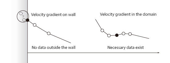
Figure 7.2: Problem with a higher-order difference method

About the Author
Takao Itami | Born in July 1973, Kanagawa, Japan

The author had conducted researches on numerical analyses of turbulence in college. After working as a design engineer for a railway rolling stock manufacturer, he took the doctor of engineering degree from Tokyo Institute of Technology (Graduate School of Science and Engineering) through researching compressible turbulent flow and Large-Eddy Simulation. He works as a consulting engineer at Software Cradle solving various customer problems with his extensive experience.