
Master Course for Fluid Simulation Analysis of Multi-phase Flows by Oka-san: 22. Liquid-liquid two-phase flow analysis with two-fluid model
Liquid-liquid two-phase flow analysis with two-fluid model
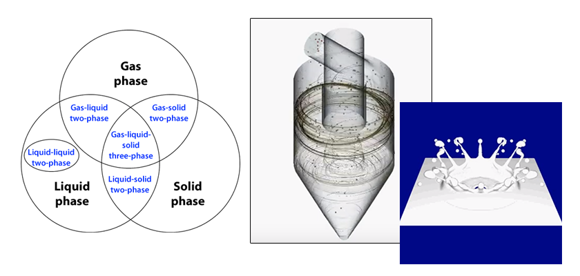
Two-fluid model is an example of gas-liquid two-phase flow analyses or liquid-liquid two-phase flow analyses. It is also called distributed multi-phase flow model, Euler-Euler model, Euler multi-phase flow model depending on the fluid simulation analysis software products, however, they are the same as a model to solve the basic equation for each phase by regarding each phase as a continuum. The model can be expanded to n-fluid model, however, analysis is possible up to three-fluid model in consideration of calculation load and convergence.
Figure 1 shows an outline figure of underwater bubble jet analysis, and Figure 2 shows the gas phase volume fraction of the analysis result. As shown in Figure 2, it is also possible to analyze by regarding the particles of flowing bubbles and liquid drops as a continuum (dispersed phase). In addition, it is possible to analyze even a solid-gas two-phase flow and a solid-liquid two-phase flow by regarding powder as a continuum. In both cases, it is necessary to define interactions between phases (resistance that the particles receives from the fluid) and between particles.
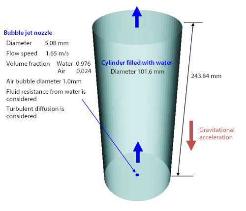
Figure 1: Underwater bubble jet analysis
Figure 2: Phase volume fraction distribution
Here is an analysis example. Different liquids are mixed with a static mixer. Since a static mixer has a simple structure and does not require rotation power, it is used in various fields. As shown in Figure 3, consider piping with a T-shape pipe (JIS 8A Sch. 20S, internal diameter of 9.8 mm). Pour two liquids with a density of 1000 kg/m3 and a viscosity of 1.0 Pa·s from two inlets at a flow rate of 0.30 L/min. The viscosity of the two liquids is 1000 times as high as that of water and same as that of fruit source. Twelve elements with a length of 10.4 mm are set by changing the angle of the straight axis direction by 90 degrees. Under these conditions, steady analysis of the laminar flow is conducted.
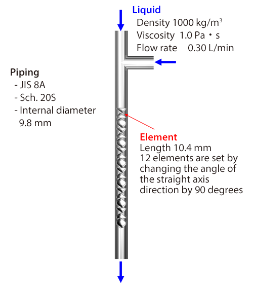
Figure 3: Static mixer
Figure 4 shows the volume fraction distribution of liquids, and Figure 5 shows a flow line map. The two liquids are represented in red and white so that they can be distinguished easily. By mixing them, the volume fraction distribution becomes more homogenized. By adding eight elements, steady analysis is conducted with 20 elements in total. As shown in Figure 6, the volume fraction distribution is almost homogenized.
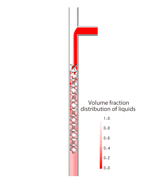
Figure 4: Volume fraction distribution of liquids (12 elements)
Figure 5: Flow lines
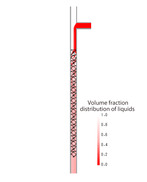
Figure 6: Volume fraction distribution of liquids (20 elements)
Now, unsteady analysis of the laminar flow is conducted by changing the material properties of two liquids. As shown in Figure 7, JIS 8A Sch. 20S is used for the piping on the straight side of the T-shape pipe, and 6A Sch. 20S (internal diameter of 7.5mm) on the mixing side. The liquid that flows straight ahead has a density of 1000 kg/m3 , viscosity of 0.001 Pa·s (same as water), and flow rate of 0.30 L/min, and the liquid that is mixed has a density of 1000 kg/m3 , viscosity of 0.0035 Pa·s, and flow rate of 0.075 L/min. Imagine that milk is added to coffee to make coffee‐flavored milk with a volume ratio of 20%. Figure 8 shows the temporal change of the volume fraction distribution. It shows that it becomes more homogenized. When the difference of material properties of the two liquids is made larger, the degree of separation increases, producing a free surface flow. In this case, it is recommended to analyze with the VOF method introduced in this column before. The time in the video in Figure 8 is accelerated by two times.
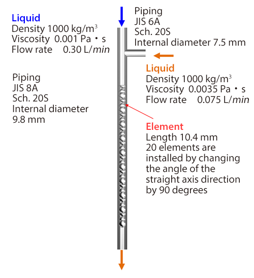
Figure 7: Static mixer with material properties of liquids changed
Figure 8: Volume fraction change of liquids
This column is concluded with this section. Thank you very much for reading this series. As long as computers continue to evolve, the application scope of fluid simulation analyses for multi-phase flows will further expand. I hope this column has triggered you to work with fluid simulation.
About the Author
Katsutaka Okamori | Born in October 1966, Tokyo, Japan
He attained a master’s degree in Applied Chemistry from Keio University. As a certified Grade 1 engineer (JSME certification) specializing in multi-phase flow evaluation, Okamori contributed to CFD program development while at Nippon Sanso (currently TAIYO NIPPON SANSO CORPORATION). He also has experience providing technical sales support for commercial software, and technical CFD support for product design and development groups at major manufacturing firms. Okamori now works as a sales engineer at Software Cradle.

