
Master Course for Fluid Simulation Analysis of Multi-phase Flows by Oka-san: 11. Particle tracking analysis V
Particle tracking analysis V
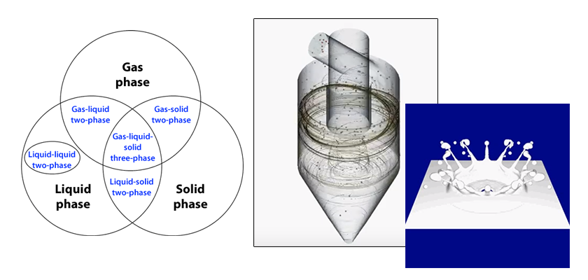
This section describes the liquefaction of particles analyzed by using the particle tracking method.
Two primary methods are used to analyze the liquefaction of particles. One is converting a particle into a liquid film as shown in Figure 1. This method will be called the “liquid film model”. In a liquid film model, the material properties (density and viscosity) and the height of a liquid film, which is generated due to the liquefaction of particles on a wall, are considered. Then, the movement of the liquid film along the wall is analyzed. The particles converted to the liquid film on the wall vanish and are no longer tracked. In this model, surface tension and contact angle are not considered. Therefore, this model is not suitable for analyzing breakup or joining of liquid films. However, the principal advantage of this model is its low calculation load.
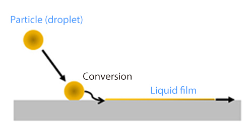
Figure 1: Liquid film model
Figure 2 shows an example of a liquid film model. Green particles (diameter: 100 μm) are sprayed from a nozzle and liquefied on a slanted black board (50 mm x 40 mm). The thickness of the sprayed liquid film is 1 mm as shown in Figure 2. In Figure 3, the model is viewed from the top of the nozzle. The sprayed particles have an elliptic shape whose major axis is 30 degrees and minor axis is 10 degrees. Note that Figure 2 and 3 are 500 times slower than the real time. This liquid film model is useful for simulating a thinly spreading liquid film on a wall. In recent years, this model has been used to analyze direct fuel injection in automotive engines.
Figure 2: Analysis example of liquid film model
Figure 3: Viewpoint from the nozzle top
The second method for analyzing particle liquefaction is combining the aforementioned method of converting particles into a liquid film with a free surface flow analysis described in previous articles (i.e. the MARS method). When particles adhere to a wall or liquid surface as shown in Figure 4, particles are converted into a liquid. Particles converted into a liquid disappear and are no longer tracked. Since surface tension and contact angle can now be considered, the breakup and joining of liquid films can be analyzed. However, the calculation load is more intensive than the load for the simpler liquid film model.
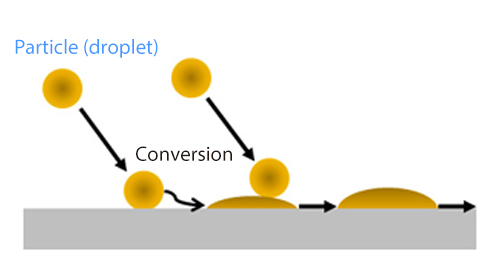
Figure 4: Combination use with free surface flow analysis
An analysis example can be used to illustrate this method. A semiconductor single-wafer cleaner is analyzed by using the particle tracking method with free surface flow analysis (MARS method). A 300 mm diameter wafer is surrounded by a circular pipe with a diameter of 372 mm. The top of the pipe is drawn into a conical shape. A spray nozzle for cleaning water is mounted 45 mm above the wafer face. Air enters the top of the conical section at 0.5 m/s and cleaning water is released downward toward the wafer.
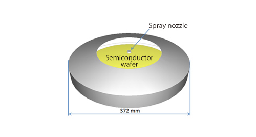
Figure 5: Single wafer cleaner
The spray nozzles used in this analysis are single-fluid nozzles. The particle diameter is 50 μm, the spray flow rate is 0.50 kg/s (30 L/min), and the spray velocity is 15 m/s. Figure 6 shows the spray pattern 35 mm from the tip of the nozzle at 0.004 seconds. Two spray patterns are used. One is a conical spray with the spray angle of 30 degrees (Left). The other is an elliptic spray with the spray angle of 5 degrees (Right). In addition, the material properties for pure water are used, and the contact angle is 50 degrees.
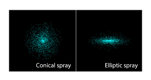
Figure 6: Analysis results (spray)
Figure 7 shows the time variation of the cleaning water for the conical spray at 0.1 seconds. The cleaning water spreads radially from the center of the wafer. Figure 8 shows the time variation of the cleaning water for the elliptic spray. Note that the time in Figures 7 – 10 is 50 times slower than real time.
Figure 7: Time variation of cleaning water for a conical spray
Figure 8: Time variation of cleaning water for an elliptic spray
For a single-wafer cleaner, a wafer is rotated at high speed to enhance the cleaning efficiency. The time variation of elliptic spray cleaning water is shown in Figure 9 and 10 where the wafer is rotated at high speeds. The wafer is rotated at 2,500 rpm and 5,000 rpm, respectively. The figures also show that the cleaning water spreads in a circumferential direction.
Figure 9: Time variation of cleaning water (Elliptic spray, 2,500 rpm)
Figure 10: Time variation of cleaning water (Elliptic spray, 5,000 rpm)

About the Author
Katsutaka Okamori | Born in October 1966, Tokyo, Japan
He attained a master’s degree in Applied Chemistry from Keio University. As a certified Grade 1 engineer (JSME certification) specializing in multi-phase flow evaluation, Okamori contributed to CFD program development while at Nippon Sanso (currently TAIYO NIPPON SANSO CORPORATION). He also has experience providing technical sales support for commercial software, and technical CFD support for product design and development groups at major manufacturing firms. Okamori now works as a sales engineer at Software Cradle.

