
Optimization: Tool for Fast, Cost-Efficient Analysis
Shigeki Katsumura (Software Cradle, Assistant Manager, Software Engineering Dept.)
Optimization: Tool for Fast, Cost-Efficient Analysis
Searching for the ideal combination of design variables and objective functions requires high level of engineering knowledge and experience; this is quite a task when there is limited time. Software Cradle’s Extension Option (Optimization) known as EOopti can cut down unnecessary trial and error and identify the most fitting variable and object combinations for each design case, all in a short amount of time. Shigeki Katsumura, Assistant Manager of the Cradle Engineering Department, explains why and how this tool was developed. 
Shigeki Katsumura, Software Cradle Co., Ltd., Assistant Manager, Software Engineering Dept.
What Motivated You to Develop this Optimization Tool?
The advancement of computer processing speed has made it much more common that product engineers apply CAE (Computer Aided Engineering) in their daily design work. As a developer of fluid analysis software, Cradle is an important contributor to not only promoting this trend but also advancing it. In particular, even as the use of CAE has become more common, there is an increasing realization that CAE has even greater potential. The ultimate desire is for the CAE analysis to encompass our experiences, knowledge, and decision-making abilities, such that the final model contains the highest level of thinking.
Optimization involves trial and error, whether developing a vehicle with the least air resistance, allocating parts, or modeling heat sinks. Thermal fluid analysis can sometimes take significant amount of time to calculate the solution depending on model shape. The ideal situation would be to identify the optimized modeling and part allocation from only a few samples. However, in reality engineers must often review hundreds and thousands of samples, before determining the best solution, which consumes time and money.
That was what inspired us to develop an optimization tool that can reduce examination tasks and identify the design variables most fitting for the customer’s purpose. After a thorough search of available optimization methods, we decided to implement MOGA (Multi Objective Generic Algorithm), which was introduced by Tohoku University’s Obayashi Laboratory, in the EOopti available from Version 10 onward.
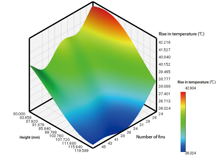
Figure 1 Response surface calculated by Kriging
What Challenges Did You Face during Development?
When I was first assigned to develop EOopti, I’d had very little experience working with optimization problems. My first struggle was to come up with a concept for the GUI (Graphic User Interface) specification. To overcome the challenge, our team worked closely to investigate prototypes, discuss how they could be improved and implement those changes; we repeated this process a number of times before reaching the final design.
The biggest issue for me was that I needed to develop a deep understanding of the optimization algorithm to create highly extensible GUI. Naturally I had to do these things concurrently – namely, developing an understanding of the algorithm, implementing the algorithm, determining the GUI specification and implementing GUI.
It was challenging, but between my research and consulting with other developers who provided much useful insight, the vision for how the application should function gradually became clear.
Tell us About the Tool Structure and How to Use it
EOopti will be displayed as shown in Figure 2. A response surface can be generated using the Kriging method. The condition wizard is used to input the necessary data to execute the multi-purpose optimization tool which implements MOGA. Optimized results will be added to the graph tree as new labels, and each graph can be viewed on a draw window.
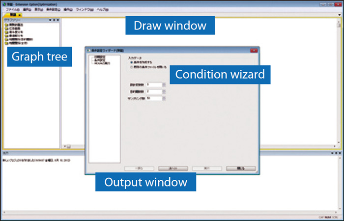
Figure 1 Response surface calculated by Kriging
The Kriging method is an interpolation technique to estimate the value at a given point based on the known values in the neighborhood of the point. Ideally we would have a mathematical expression for the optimizing target, i.e. each objective function value, but working with non-linear substances like fluid makes the process extremely complicated. As an alternative approximation to each objective function, EOopti applies the Kriging method, based on the sampling point, to generate the response surface distribution and then runs MOGA to find the optimized solution.
The process to determine the optimum solution can be divided into the following three phases:
- Define the design variables and objective functions
- Generate the sampling point (design variable value)
- Specify the objective function value based on the design variable value from phase 2.
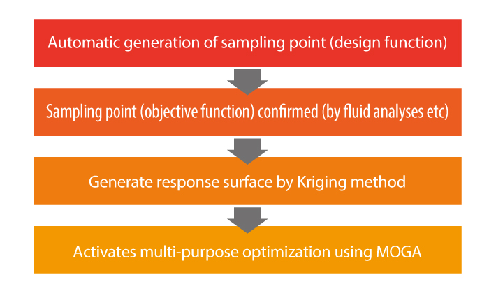
Figure 3 Optimization workflow using EOopti
Phases 1 and 2 can be carried out in EOopti, whereas phase 3 requires values from additional information, including data from the analysis results.
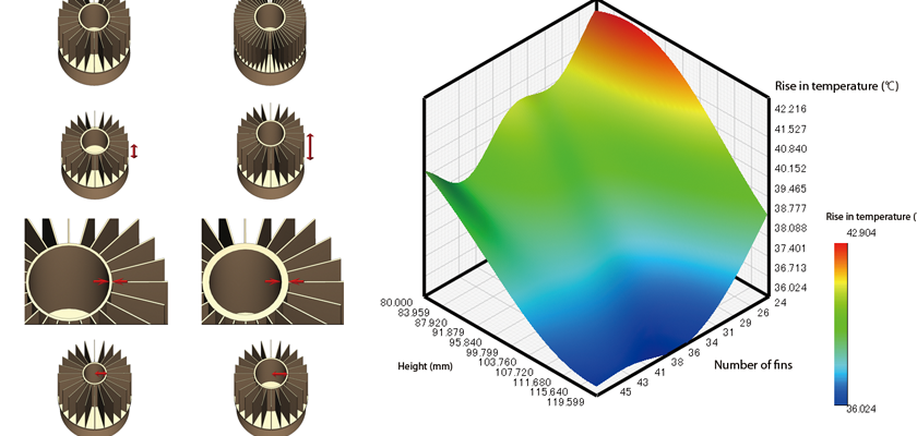
An example of a heat sink can be used to illustrate the process. The heat sink dissipates heat inside an LED lamp as shown in Figure 4. Optimization in this case involves the following design variables: the number of fins, fin height, thickness of the heat sink shaft, and the outer diameter of the fin and shaft sections. The objective function values are based on the LED temperature and volume. The range of each design variable is shown in Figure 5.
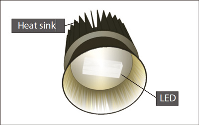
Figure 3 Optimization workflow using EOopti
1) Define the design variables and objective functions
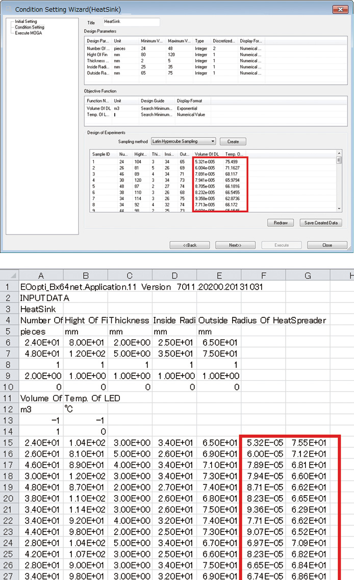
Setting EOopti conditions can be done using the condition wizard (Figure 6). On the first page of the condition wizard, engineers input values for the design variables, objective functions and sampling point. In this case, the design variable is 5, the objective function is 2, and the sampling point is 50. These values simply mean that analysis results are necessary for 50 cases, and the results will be used to generate the response surface using the Kriging method.
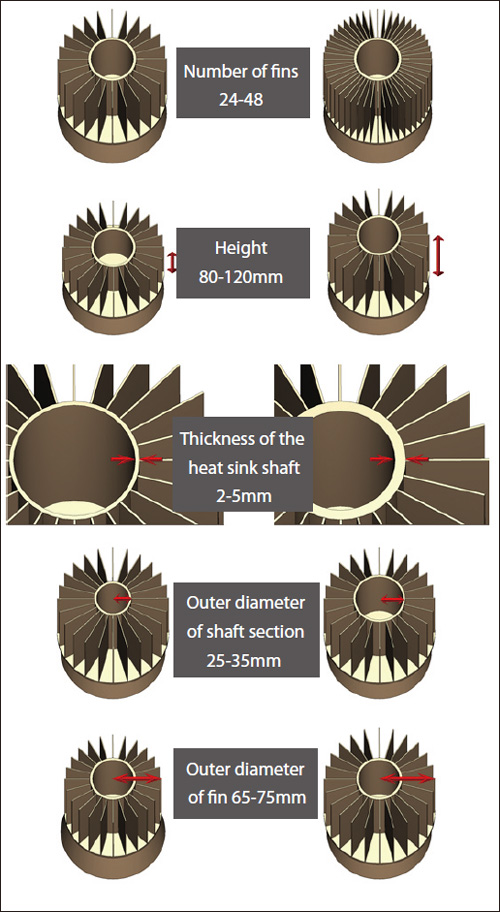
Figure 5 Range of design variables
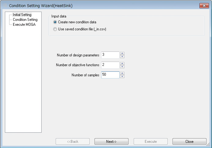
Figure 6 Condition wizard
2) Generate the sampling point (design variable values)
Engineers input data for the design variable range, design guidelines for objective functions (whether to target the maximum value or the minimum value) and sampling point. For design variable sampling, EOopti applies Latin hypercube sampling, which can be activated by clicking ‘generate.’ This calculates the design variable values automatically (Figure 7).
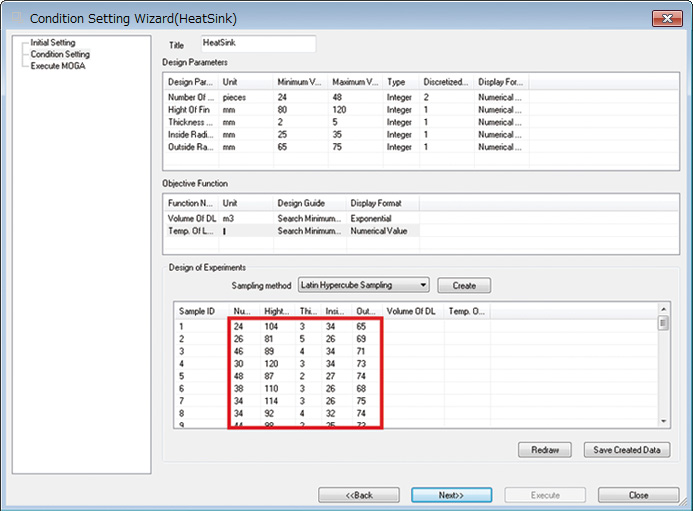
Figure 3 Optimization workflow using EOopti
3) Specify the objective function value based on the design variable value from step 2
In this section, engineers input objective function values into the blank space in condition wizard. They are the values from the LED lamp volume calculated by the design variables at the original sampling point - and the temperature results from the scSTREAM analysis (Figure 8). Values can be both imported and exported in CSV format, allowing users to input the objective functions in Excel or other editing software, and to import the data into EOopti from there (Figure 9).
Above: Figure 8 Condition wizard
Below: Figure 9 Objective functions inputs using Excel
This completes setting up the problem. Clicking ‘execute’ activates the optimization, which implements the Kriging method and MOGA (Figure 10).
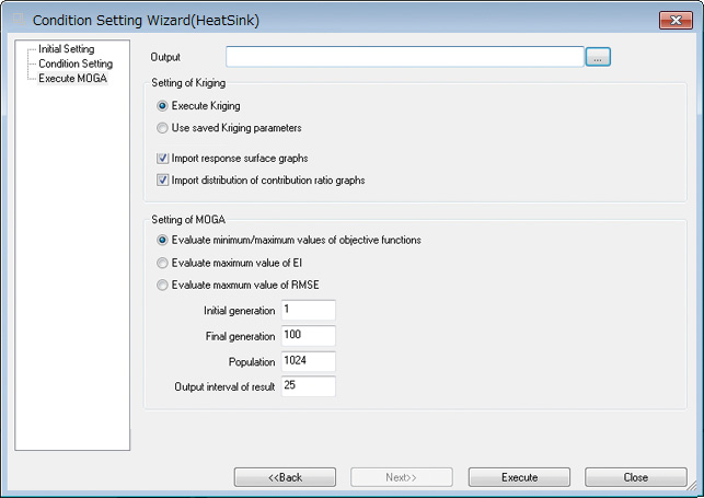
Figure 10: Condition wizard
When optimized, engineers can view the response surface (Figure 1, distribution of contribution, distribution of optimum solutions calculated by MOGA (Figure11), and correlation graph (Figure 12) on the draw window.
Throughout these steps data can be input manually, although this is time consuming especially when generating and inputting sample values for the objective functions. This time consuming process can be streamlined by applying VBA available from Microsoft® and Office products, or Cradle’s VBI for SC/Tetra and scSTREAM. Using these ancillary software products the entire system can be constructed and the entire process automated, from fluid analysis to optimization.
What EOopti Offers
This multi-purpose optimization can generate the distribution of the optimum solutions as shown in Figure 11. While EOopti may not be the best way to identify the single local optimum solution, its greatest advantage is its capability to quickly find several possible optimum solutions. A group of optimum solutions for the objective functions generated for a fixed value, the so-called Pareto front, can be viewed by the curve on the distribution of the optimum solution. By rapidly generating this kind of information, EOopti helps reduce the overall time and cost.
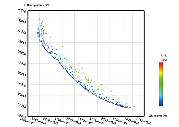
Figure 11: Distribution of optimum solutions calculated by MOGA
One thing to note is that the optimized values will be less reliable if the response surface is not accurate. This is because the response surface model from the Kriging method is only an alternative approximation. To promote certain accuracy, accurate design variable values for the sampling point should be used. This is especially important when fluids are involved. A large number of meshes and adjustments to the setting conditions may be necessary to accurately represent real phenomena. This means use of parallel solvers and sufficient computing horsepower will be helpful to generate accurate results in as short a time as possible.
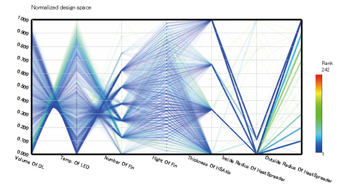
Figure 12: Correlation calculated by MOGA
Promising Future of EOopti
EOopti is a new tool, which has only been available from Version 10. It is still at its early phase and will continue to be improved as an even more convenient optimization tool.
*All product and service names mentioned are registered trademarks or trademarks of their respective companies.
*Contents and specifications of products are as of January 1, 2013 and subject to change without notice. We shall not be held liable for any errors in figures and pictures, or any typographical errors.
Download

