Particle tracking method VI

This article uses an analysis example to illustrate how to apply external forces to particles using the particle tracking method.

Fluid simulation analysis software must often be able to apply external forces, other than gravity, to particles in a fluid. Most software products incorporate user-defined functions to apply the external forces to particles. Today, several products can model external forces as purchased.

Static electricity is a frequently considered external force. Electrostatic painting and removal of static electricity are technologies used in various fields. To model static electricity using the particle tracking method, the electric potential distribution of the fluid must be obtained (Figure 1). Figure 1 shows analysis result for the electric potential distribution of water (Relative permittivity: 80.4) in a square with side lengths of 60 mm. The voltages at the centers of upper and lower faces are set to 0 V and -100 V, respectively. The arrows in the figure represent the electric flux density. Particles to which the electric charge will be added (charged particles) are tracked after the electric flux density of the fluid is obtained.

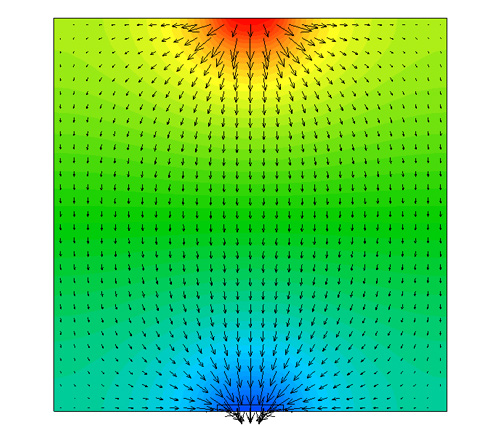
Figure 1: Electric potential distribution of a fluid

 
The electrostatic force (Coulomb force) is treated as an external force. Figure 2 shows the behavior of uncharged particles analyzed using two way coupling. In a two way coupling, the interactions between both the fluid and the particles are considered. The particles’ repulsion coefficient at a boundary is 1. Figure 3 shows the analysis result for particles with an electric charge of -0.1 nC (nano coulomb). The particles are repulsed by the upper surface but attracted to the center of the upper surface by electrostatic forces.

Figure 2: Behavior of uncharged particles  

Figure 3: Behavior of charged particles  

This analysis example will demonstrate a practical application. A spray gun used to electrostatically apply a coating is analyzed using the particle tracking method.

A coating booth has a length (L) of 500 mm, width (W) of 300 mm, and height (H) of 250 mm (Figure 4). The coating target is an icosagon-based prism with L of 20 mm and H of 200 mm. The prism is located 100 mm away from the tip of the electrostatic spray gun. The air flows into the booth from the ceiling with a velocity of 0.3 m/s. The air is used to remove paint particles that have not adhered to the prism. The floor of the booth is the outlet. It is a grating floor. The electric flux density for all the walls of the booth, including the ceiling and the floor, is set to 0 C/m². The electric potential of the prism is set to 0 V (the ground potential). The relative permittivity of the air is 1.000586.

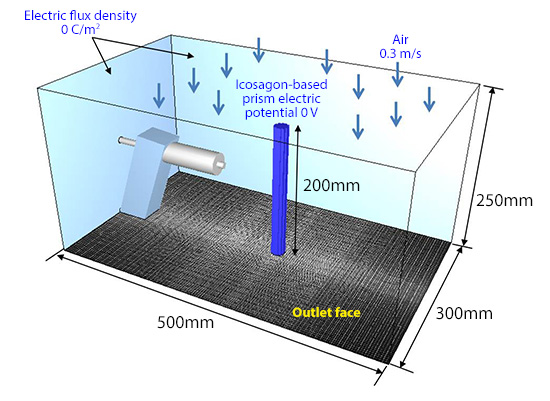
Figure 4: Coating booth
 

The air flow rate from the electrostatic spray gun is 40 L/m (Diameter of the nozzle: 10 mm), and the paint spray rate is 100 g/min (Density of the paint: 1,000 kg/m³ ). (See Figure 5.) The paint particle diameter is 50 μm. The parcel approximation is applied and one parcel consists of approximately 5 particles of paint.

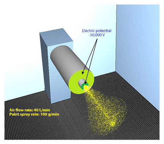
Figure 5: Electrostatic spray gun
 

The electric potential at the tip of the nozzle is -50,000 V. In addition, the electrical potential at the front face of the gun body (indicated in light green in the figure) is set to -50,000 V to prevent paint from accumulating on the gun body. Particles that adhered to the prism are treated as having “vanished” and their motion is not tracked any longer. The vanished particles accumulate and are converted to the thickness of the paint film. In this analysis, the mobility of the paint film is not considered.

Figure 6 shows the electric potential distribution at the central cross section. (Its lower limit is set to -17,000 V.) The dotted line in the figure indicates the electric flux density.

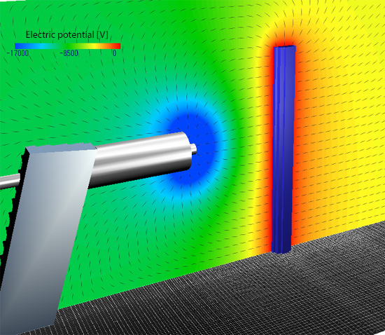
Figure 6: Electric potential distribution
 

The paint film thickness distribution on the prism for uncharged particles is shown in Figures 7 and 8. The upper limit of the thickness is set to 10 μm. A paint film from uncharged particles does not form on the side and back faces of the prism as shown in Figure 8.
 

Figure 7: Distribution of the paint film on the front face of the prism (Without charge)

 

Figure 8: Distribution of the paint film on the back face of the prism (Without charge)

Figures 9 and 10 show the paint film thickness distribution for particles charged at 1.0 pC (pico coulomb). Figure 10 shows that the paint film from charged particles is generated on the side and back surfaces of the prism due to static electricity.
 

Figure 9: Distribution of the paint film on the front face of the prism (With charge)

 

Figure 10: Distribution of the paint film on the back face of the prism (With charge)
 

The coating efficiency of the paint spray process is calculated from the number of paint particles that adhere to the prism divided by the number of particles sprayed from the nozzle. The calculated spray efficiency is 60% without electrostatics. It is 85% with electrostatics. These results are in the range of expected efficiency improvements when electrostatics is used and shows that the effect of electrostatic painting has been simulated well. In the animation of Figures 7 to 10, the motion is 100 times slower than the real phenomena.

This is the last article discussing the particle tracking method. These articles have shown that physical phenomenon such as mass particles, reactive particles, charged particles, and evaporation/volatilization/liquefaction of particles can be computationally simulated using the particle tracking method. This method can be used for many different kinds of particle analyses.

---

About the Author 
Katsutaka Okamori | Born in October 1966, Tokyo, Japan

He attained a master’s degree in Applied Chemistry from Keio University. As a certified Grade 1 engineer (JSME certification) specializing in multi-phase flow evaluation, Okamori contributed to CFD program development while at Nippon Sanso (currently TAIYO NIPPON SANSO CORPORATION). He also has experience providing technical sales support for commercial software, and technical CFD support for product design and development groups at major manufacturing firms. Okamori now works as a sales engineer at Software Cradle.